(Importance Weighted) Variational Autoencoders Derived

Variational Autoencoders

Let $x$ denote a random variable which is generated by a random process. This random process first samples a random latent variable $z$ and subsequently generates $x|z \sim p(x|z)$ by conditioning the random process $p(x|z)$ on the random variable $z$. Thus we are dealing with a generative model which can generate valid samples $x$ from some random $z$. We are interested in the latent distribution of $p(z |x)$ given the data $x$ and wish to learn it. Intuitively, we want to know for a given $x$ what the latent variables $z$ were that generated them. This is akin to observing some observation $x$ and being able to say: I know the $z$ ‘s that generated that!.

By Bayes rule we now that for a distribution $ p ( x | z ) $ there also exists the distribution $ p ( z | x ) $, the distribution we are interested in. \(\begin{align} p(z|x) = \frac{p(z,x)}{p(x)} = \frac{p(x|z)p(z)}{p(x)} \end{align}\) The crux of the problem is that we can only observe the data distribution $p(x)$ through a data set $\mathcal{D}= \{ x_i \}_{i=0}^N$. So we neither know what form the data generating process $p(x|z)$ has nor what the true latent distribution $p(z)$ is. Additionally, the data probability $p(x)$ is even more obscure. How would you even answer the question of how probable your data set is?

What we do know is the following: We want to find a variational distribution, let’s name it $q_\phi(z |x)$ with the optimizable parameters $\phi$, which we want to be as close as possible to the true distribution $p(z |x)$. The motivation behind this formulation is that the true latent conditional distribution $p(z|x)$ could be very complicated, but we will choose a simpler variational distribution $q_\phi(z |x)$ that we can conveniently work with. It might not be able to represent all the modes and fat tails that could potentially occur in $p(z |x)$ but better than nothing, right?

Information theory gives us the right tools to measure the difference between $q_\phi(z|x)$ and $p(z|x)$ through the Kullback-Leibler divergence: \(\mathbb{KL} \left[ q_\phi(z|x) \ || \ p(z|x) \right]\) The state of affairs sofar is that we have an easy to work with distribution $q_\phi(z|x)$ with the trainable parameters $\phi$ and that we wish to minimize the divergence to the true latent distribution $p(z|x)$. We can also rewrite $p(z|x)$ according to Bayes rule to maybe make the computations a bit more tractable. We can now write out the Kullback-Leibler divergence and inspect the terms that arise from some algebraic manipulation:

\(\begin{align} \mathbb{KL} \left[ q_\phi(z \| x) \ || \ p(z \| x) \right] &= \mathbb{E}_{q_\phi(z \|x)} \left[ \log \frac{q_\phi(z \| x)}{p(z \| x)} \right] \\ &= \mathbb{E}_{q_\phi(z|x)} \left[ \log q_\phi(z|x) - \log p(z|x)\right] \\ &= \mathbb{E}_{q_\phi(z|x)} \left[ \log q_\phi(z|x) - \log \frac{p(z,x)}{p(x)}\right] \\ &= \mathbb{E}_{q_\phi(z|x)} \left[ \log q_\phi(z|x) - \log p(z,x) + \log p(x)\right] \end{align}\) From earlier we know, that the data marginal probability $p(x)$ is almost surely intractable so we might want to avoid working with it directly. But by applying Bayes’ rule we suddenly see that we are working with the joint probability $p(z,x)$. Given the fact that $0 \leq \mathbb{KL}$ we can deduce \(\begin{align} 0 &\leq \mathbb{KL} \left[ q_\phi(z|x) \ || \ p(z|x) \right] \\ 0 &\leq \mathbb{E}_{q_\phi(z|x)} \left[ \log q_\phi(z|x) - \log p(z,x) + \log p(x) \right] \\ 0 &\geq \mathbb{E}_{q_\phi(z|x)} \left[ -\log q_\phi(z|x) + \log p(z,x) - \log p(x) \right] \\ \log p(x) &\geq \mathbb{E}_{q_\phi(z|x)} \left[ - \log q_\phi(z|x) + \log p(z,x)\right] \\ \log p(x) &\geq \mathbb{E}_{q_\phi(z|x)} \left[ - \log q_\phi(z|x) + \log p(x|z) p(z)\right] \\ \log p(x) &\geq \mathbb{E}_{q_\phi(z|x)} \left[ - \log q_\phi(z|x) + \log p(x|z) + \log p(z)\right] \\ \log p(x) &\geq \mathbb{E}_{q_\phi(z|x)} \left[ \log \frac{p(z)}{q_\phi(z|x)} + \log p(x|z) \right] \\ \log p(x) &\geq -\mathbb{E}_{q_\phi(z|x)} \left[ \log \frac{q_\phi(z|x)}{p(z)} \right] + \mathbb{E}_{q_\phi(z|x)} \left[ \log p(x | z) \right] \\ \log p(x) &\geq -\mathbb{KL} \left[ q_\phi(z|x) || p(z) \right] + \mathbb{E}_{q_\phi(z|x)} \left[ \log p(x|z) \right] \end{align}\) What does the inequality above tell us? It says that if we want to maximize the probability of the data we must minimize the KL divergence in the first term and maximize the probability of the generative model $p(x|z)$. So for any given $z$, we want the generative model $p(x|z)$. If we optimize the two terms on the right, we will obtain an inference model $q_\phi(z|x)$ which inverts the generative model $p(x|z)$.

The problem, though, is that we have no clue what either $p(z)$ nor the true generative model $p(x|z)$ actually is. Here comes the fun part: Let’s just assume stuff and parameterize both $p(z)$ and $p(x|z)$ such that we can easily and conveniently work with them. Since $p(z)$ is a latent distribution we will enforce a strong simplicity by assuming that it follows a standard normal distribution $\mathcal{N}(0, I)$. We could assume any other family of distributions but the standard normal distribution has lots of nice perks and properties. This might seem bold but if the generative model $p(x|z)$ is flexible enough it can generate any $x$ from this comparatively simpel $z$. Now let’s turn our attention to $p(x|z)$: We will change the unknown $p(x|z)$ to a parameterized and differentiable $p_\theta(x|z)$ such that we can maximize the probability of the data $x$ for a given $z$.

Now we have the following objective function: \(\begin{align} \log p(x) \geq -\mathbb{KL} \left[ q_\phi(z|x) || p(z) \right] + \mathbb{E}_{q_\phi(z|x)} \left[ \log p_\theta(x|z) \right] \end{align}\) which, upon closer inspection, has a lot of similarities to an autoencoder, except that it’s probabilistic! We use the distribution $q_\phi(z|x)$ to infer some latent code from a given sample. Through the KL divergence we enforce that the latent representation should be close to the simplified assumption of $p(z) = \mathcal{N}(0,I)$. The same latent code $z$ should be reconstructed to the true sample $x$ by the generative model $p_\theta(x|z)$. So we can actually interpret $q_\phi(z|x)$ as a probabilistic encoder and $p_\theta(x|z)$ as a decoder.

It is important to note that the prior and data loglikelihood are not balanced with respect to the data set size as it is done in Bayesian neural network and the parameter prior. The KL divergence between the latent code $q_\phi(z|x)$ and the prior $p_\theta(z)$ is computed for each data point independently and is equally balanced.

Jensen’s Inequality

The core idea of variational autoencoders and, to a larger extent, variational inference is that we optimize the $ \mathbb{E} [ \log p(x|z) ]- \mathbb{KL} [ q(\theta) || (p(\theta) ] $ in the hopes that we are able to push the bound as close as possible to the true value $\log p(x)$. The ELBO can thus be understood as a surrogate criterion.

The derivation of the ELBO originates from the minimization of the Kullback-Leibler divergence. It turns out that we can also derive an alternative criterion in order to maximize $\log p(x)$, the term we ultimately want to see maximized. In order to derive this alternative bound we will first have to understand Jensen’s inequality.

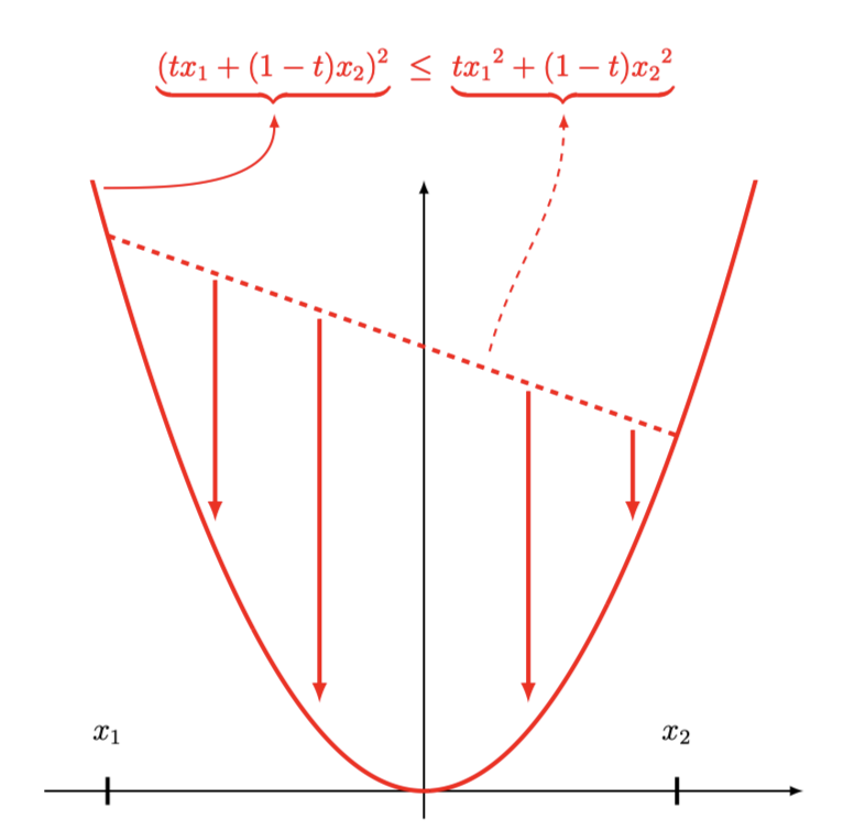
Let’s assume that we have the quadratic function $f(x) = x^2, x,y \in \mathbb{R}$. The quadratic function is convex which is essential for Jensen’s inequality. For any convex function $f(x)$, Jensen’s inequality for $t \in (0,1)$ states: \(\begin{align} f(tx_1 + (1-t) x_2 ) \ \leq \ t \ f(x_1) + (1-t) \ f(x_2) \end{align}\) which is the definition of a convex function and quintessentially asks the question of whether we interpolate the function values $f(x)$ or interpolate the arguments $x_1$ and $x_2$.

Interpolating the function values $f(x)$ results in a straight line from $f(x_1)$ to $f(x_2)$. Interpolating the arguments results in tracing the original function $f(x)$. Since the quadratic function in its vanilla form is convex, we can conclude that interpolating the arguments will always be below the interpolation of the function values.

Jensen’s inequality becomes useful for deriving bounds when applied to probability theory. We can expand the interpolation beyond the two values $x_1$ and $x_2$ by weighting the values uniformly: \(\begin{align} f\left( \frac{1}{2} x_1 + \frac{1}{2} x_2 \right) \ \leq \ \frac{1}{2} \ f\left( x_1 \right) + \frac{1}{2} \ f \left( x_2 \right) \end{align}\) We can then extend the interpolation to $x_n \in \{x_1, \ldots, x_N \}$ via \(\begin{align} f\left( \frac{1}{N} x_1 + \ldots + \frac{1}{N} x_N \right) \ & \leq \ \frac{1}{N} \ f\left( x_1 \right) + \ldots + \frac{1}{N} \ f \left( x_N \right) \\ f\left( \frac{1}{N} \sum_n^N x_n \right) \ & \leq \ \frac{1}{N} \sum_n^N \ f\left( x_n \right) \\ \end{align}\) which gives us the probabilistic version of Jensen’s inequality for a convex function $f(x)$: \(\begin{align} f \left( \mathbb{E}[x_n] \right) \ & \leq \ \mathbb{E} \left[ f(x_n) \right] \\ \end{align}\)

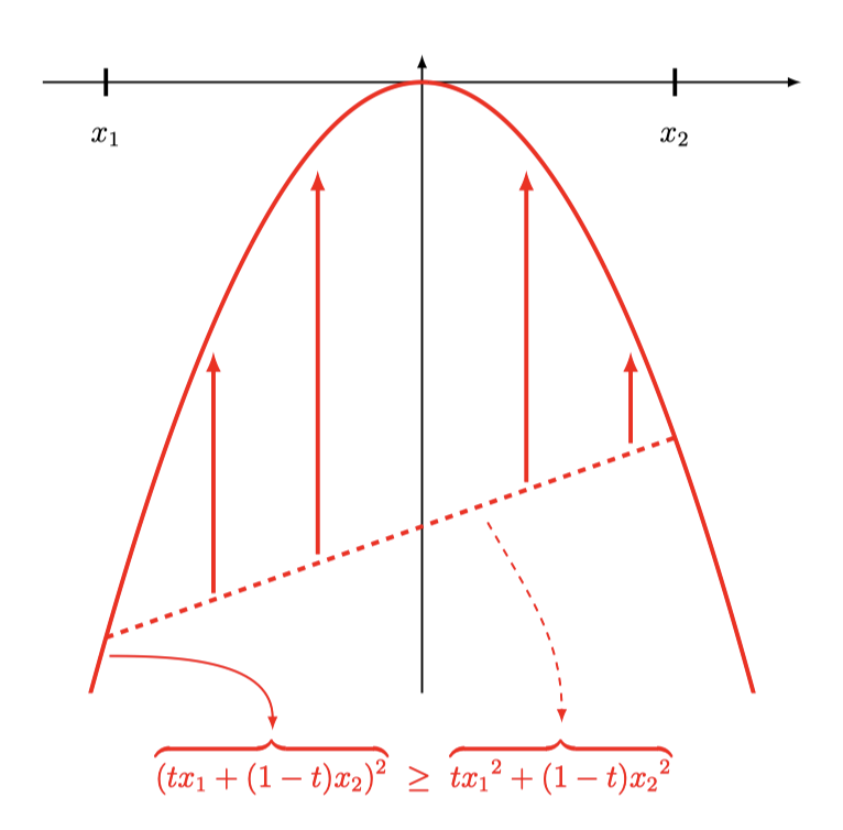
For a concave function, we simply have to flip the inequality sign, as the function value interpolation $\mathbb{E}[f(x)]$ will always be equal or below the argument interpolation $f(\mathbb{E})[x]$: \(\begin{align} f \left( \mathbb{E}[x_n] \right) \ & \geq \ \mathbb{E} \left[ f(x_n) \right] \\ \end{align}\)

Importance Weighted Variational Autoencoders

To derive the loss for the Importance Weighted Variational Autoencoder we will use two tricks: the fact that the logarithm is a concave function and utilizing importance sampling. \(\begin{align} \log p(x) &= \log \left[ \int p(x| z) p(z) dz \right] \\ &= \log \left[ \int q(z|x) \frac{p(x|z) p(z)}{q(z|x)} dz \right] \qquad \Leftarrow \text{expanding with $\frac{q(z|x)}{q(z|x)}$} \\ &= \log \left[ \mathbb{E}_{q(z|x)} \left[ \frac{p(x|z) p(z)}{q(z|x)} \right] \right] \\ &\geq \mathbb{E}_{q(z|x)} \left[ \log \left[ \frac{p(x|z) p(z)}{q(z|x)} \right] \right] \qquad \Leftarrow \text{pulling in $\log$ with Jensen's inequality = ELBO} \end{align}\) and we arrive at the original ELBO derived from the Kullback-Leibler divergence from the original VAE formulation.

The important step is applying Jensen’s inequality where we introduce the bound for the first time. If we leave the expectation in the log we are still working with marginal data log-likelihood instead of the bound. Only after applying Jensen’s inequality do we loosen the equality to an inequality which is the ELBO.

The remedy to fending off the loose ELBO is given by evaluating the term before applying Jensen’s inequality by pulling in the logarithm. This gives us an importance sampling algorithm which repeatedly samples $z \sim q(z|x)$ and subsequently evaluating $p(x|z)$. This tightens the bound and we have better criterion.

Squeezing Jensen

We stated earlier, that if we apply Jensen’s inequality and sample $z$ once, we have the original training procedure of the VAE. But the latent representation is a distribution so why should we only sample once? Probably because we’re lazy and stochastic optimization theory guarantees an unbiased gradient, so if we train long enough we will arrive at the optimum. But there is no real argument against sampling multiple times from the latent distribution and averaging the reconstruction $p(x|z)$ to integrate out the randomness that is injected into the optimization through the latent distribution $q(z|x)$.

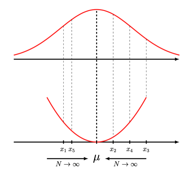
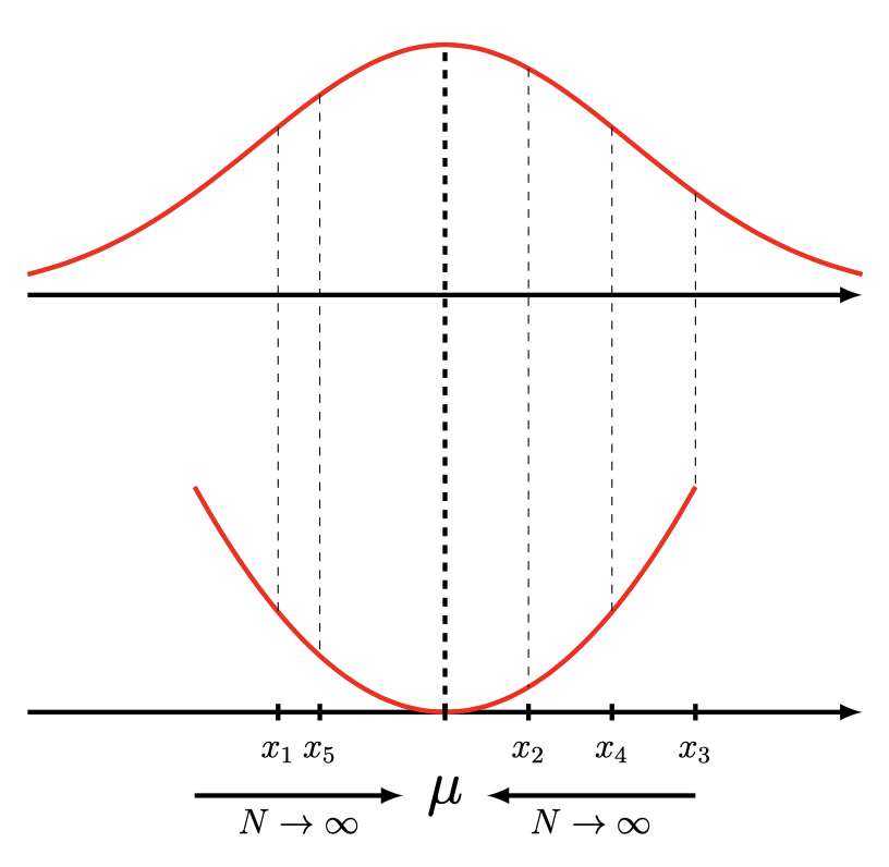
The more samples we draw, the tighter our bound becomes. Why is this the case we might ask? We take our toy example with the quadratic function again to visualize what’s happening when we draw more samples from the latent distribution \(\begin{align} f\left( \mathbb{E}[x] \right) &\leq f \left( \frac{1}{N} \sum_n x_n \right) \\ f\left( \mu \right) &\leq f \left( \frac{1}{N} \sum_n^N x_n \right) \end{align}\)

If we evaluate a finite number of samples $x_n$, the mean estimator will have a higher variance. There might be occurences where we draw the perfect sample right or very, very close to $\mu$, but on average the mean estimator will have the estimator variance \(\begin{align} \mathbb{V} \left[ \frac{1}{N} \sum_n^N x_n \right] &= \frac{1}{N^2} \sum_n^N \mathbb{V}[x] \\ &= \frac{1}{N} \mathbb{V}[x] \\ \end{align}\)

with means that \(\begin{align} f\left( \mu \right) \leq f \left( \frac{1}{N+1} \sum_n^{N+1} x_n \right) \leq f \left( \frac{1}{N} \sum_n^N x_n \right) \end{align}\) for a convex function $f(\cdot)$. Conversely for a concave function, we would have to flip the inequality sign.

By simply drawing more samples $N$ we reduce the variance and thus tighten the bound of the estimator. Visually, sampling more samples $x_n$ in the figure above asymptotically lets the estimated mean converge on the true mean. The closer the estimated mean is, the tighter the bound. This is precisely whats happening when we draw more samples in the expectation of the importance weighted VAE.

Finally, for we can use the probabilistic version of Jensen’s inequality to derive the positive constraint of the variance of a random variable $x$: \(\begin{align} \mathbb{E}[x]^2 &\leq \mathbb{E}[x^2] \\ 0 &\leq \mathbb{E}[x^2] - \mathbb{E}[x]^2 = \mathbb{V}[x] \end{align}\)