Stein's Lemma for Trace Estimation

\(\def\tr#1{\text{Tr}\left[ #1 \right]} \def\Efunc#1{\mathbb{E}\left[ #1\right]} \def\Efuncc#1#2{\mathbb{E}_{#1}\left[ #2 \right]}\)

The Trace of a Matrix

For a square matrix $A \in \mathbb{R}^{d \times d}$ the trace is defined as \(\begin{align} \tr{A} = \sum_i^d A_{ii} \end{align}\) which sums over the diagonal terms of the matrix $A$. Plain and simple.

Hutchinson’s Stochastic Trace Estimation

By definition we are only interested in the diagonal terms of a matrix when computing the trace of it. But in cases where the matrix is computationally expensive to compute we might want to approximate it.

Given a matrix $A$ one might think why the stochastic estimation is necessary when all we need to do is sum up the diagonal terms. But Hutchinson’s trick can unfold its full potential when leveraging the specific structure of the matrix $A$. Just wait until the Jacobian joins the party down below.

We can approximate the exact trace with a stochastic estimate. We therefore sample from $Z \in \mathbb{R}^D$, the mean of which is a zero vector and the covariance matrix is a identity matrix, i.e. $\Sigma[Z] = I$. More precisely we determine the covariance matrix as \(\begin{align} \Sigma[Z] &= \Efunc{(z - \Efunc{Z})(z - \Efunc{Z})^T}\\ &= \Efunc{zz^T} - \Efunc{Z} \Efunc{Z}^T \\ &= \Efunc{zz^T} \\ &= I \end{align}\)

The Rademacher distribution which samples from the set ${-1, +1}$ with equal probability offers the lowest estimator variance and is commonly used in the trace estimation trick for this reason. \(\begin{align} \text{Tr}[A] &= \text{Tr}[I A] \\ &= \text{Tr}[\Efuncc{z \sim p(z)}{z z^T} A] \\ &= \Efuncc{z \sim p(z)}{\text{Tr}{z z^T A}} \\ &= \Efuncc{z \sim p(z)}{\text{Tr}{z^T A z}} \\ &= \Efuncc{z \sim p(z)}{z^T A z} \\ \end{align}\)

where the trace operator disappears as $z^T A z \in \mathbb{R}$ is a scalar value for which the trace is a superfluous operation.

For estimating the trace of the Jacobian, we can circumvent the quadratic nature of the Jacobian by reducing the network output with a random vector z to a scalar, which can then be readily derived with a single backward pass. \(\begin{align} \text{Tr}[J_f(x)] &= \Efuncc{z \sim p(z)}{z^T J_f(x) z} \\ &= \Efuncc{z \sim p(z)}{z^T \nabla_x [f(x)^T] z} \\ &= \Efuncc{z \sim p(z)}{z^T \nabla_x [f(x)^T z] } \\ \end{align}\)

The important piece of information lies with the contraction $f(x)^T x$ which is an inner product. Naively in equation (12), we would compute the full Jacobian matrix $J_f(x)$ and then contract it. But since $z$ is a constant quantity for each sample in the expectancy, we can instead interpret $z$ as a constant scaling factor in the derivation of each output to each input which so happens to contract the full matrix. You can think of it as a inner product of random vectors in which the Jacobian matrix provides the metric tensor. So instead of Jacobian matrix times vector, we suddenly have a derivative of the scalar $J_f(x)^T z$. The Jacobian evaluation $J_f(x): \mathbb{R}^\mathcal{X} \rightarrow \mathbb{R}^{\mathcal{X}\times \mathcal{Y}}$ reduces to the stochastic $\nabla_x [ f(x)^T z ]: \mathbb{R} \rightarrow \mathbb{R}^\mathcal{X}$. Thus we saved us a lot of computations. There is obviously a price to pay, namely that we’re working with stochastic evaluations which introduces the curse of dimensionality into our evaluation.

Stein is entering the picture

Let $X \in \mathbb{R}^N$ be a normally distributed random variable $p(x) =\mathcal{N}(x ; \mu, \sigma^2)$ with mean $\mu$ and variance $\sigma^2$. Let the derivative of the normal distribution with respect to $x$ be \(\begin{align} \partial_x p(x) &= \partial_x \left[\frac{1}{\sqrt{2\pi} \sigma} e^{-\frac{(x-\mu)^2}{2\sigma^2}} \right]\\ &= -\frac{(x-\mu)}{\sigma^2} \frac{1}{\sqrt{2\pi} \sigma} e^{-\frac{(x-\mu)^2}{2\sigma^2}} \\ &= - \frac{(x-\mu)}{\sigma^2} p(x). \end{align}\) Integration by parts (IbP) serves as a inverse of the product rule $\partial_x [u(x) v(x)] = \partial_x u(x) v(x) + u(x) \partial_x v(x)$ namely \(\begin{align} [u(x)v(x)]_{x=-\infty}^{\infty} &= \int_{x=-\infty}^{\infty} u(x) \partial_x v(x) + \partial_x u(x) v(x) dx \\ &= \int_{x=-\infty}^{\infty} u(x) \partial_x v(x) dx + \int_{x=-\infty}^{\infty} \partial_x u(x) v(x) dx \end{align}\) which yields the often used identity \(\begin{align} \int_{x=-\infty}^{\infty} u(x) \partial_x v(x) dx &= [u(x)v(x)]_{x=-\infty}^{\infty} - \int_{x=-\infty}^{\infty} \partial_x u(x) v(x) dx. \end{align}\) In practice, the property that either $u(x)$ or $v(x)$ or both evaluate to zero at $x = \pm \infty$ as it is the case with common probability distributions is leveraged as an algebraic trick to ‘switch the derivative to the other function’.

Given a function $g(x)$ we can obtain a gradient estimator with the following steps via integration by parts \(\begin{align} \Efuncc{p(x))}{g(x) ( x - \mu)} &= \int g(x) (x-\mu) \frac{1}{\sqrt{2\pi} \sigma} e^{-\frac{(x-\mu)^2}{2\sigma^2}} dx\\ &= \int g(x) (x-\mu) \frac{-\sigma^2}{-\sigma^2}\frac{1}{\sqrt{2\pi} \sigma} e^{-\frac{(x-\mu)^2}{2\sigma^2}} dx \\ &= -\sigma^2 \int g(x) \underbrace{\frac{(x-\mu)}{-\sigma^2}\frac{1}{\sqrt{2\pi} \sigma} e^{-\frac{(x-\mu)^2}{2\sigma^2}}}_{\partial_x p(x)} dx \\ &= - \sigma^2 \underbrace{\int g(x) \partial_x p(x) dx}_{\text{IbP}} \\ &= -\sigma^2 \big\{ \underbrace{[ g(x) p(x)]_{x=-\infty}^{\infty}}_{p(\pm \infty)=0} - \int \partial_x g(x) p(x) dx \big\} \\ &= \sigma^2 \int \partial_x g(x) p(x) dx \\ &= \sigma^2 \Efuncc{p(x)}{\partial_x g(x)} \end{align}\)

Trace Estimation with Stein’s Lemma

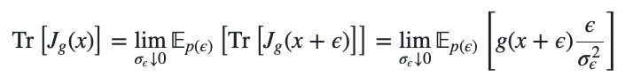
By choosing a perturbation $\epsilon \sim p(0, \sigma_\epsilon^2)$ with zero mean and a small variance $\sigma_\epsilon^2$ we can define a perturbed data point $x’ \sim p(x,\sigma_\epsilon^2)$ via $x’ = x + \epsilon$. This transforms Stein’s lemma into \(\begin{align} &\Efuncc{p(\nu))}{g(x') ( x' - x)} = \Efuncc{p(\epsilon))}{g(x + \epsilon) \epsilon} = \sigma_\epsilon^2 \Efuncc{p(\epsilon)}{\partial_{x'} g(x')}. \end{align}\) In practice we rescale with $1/\sigma_\epsilon^2$ and evaluate the left side of the following identity \(\begin{align} \Efuncc{p(\epsilon)}{g(x + \epsilon) \frac{\epsilon}{\sigma_\epsilon^2}} = \Efuncc{p(\epsilon)}{\partial_{x+\epsilon} g(x+\epsilon)}. \end{align}\) which gives us an estimator of the gradient $\partial_x g(x)$ by averaging the gradients in the $\epsilon$-neighborhood of $x$. For a function $g: \mathbb{R}^M \rightarrow \mathbb{R}^N$, the gradient estimation with Stein’s lemma estimates the trace of the Jacobian $J_g(x+\epsilon)$ \(\begin{align} \Efuncc{p(\epsilon)}{g(x + \epsilon) \frac{\epsilon}{\sigma_\epsilon^2}} = \Efuncc{p(\epsilon)}{\text{Tr}\left[ J_g(x+\epsilon)\right]}. \end{align}\) In the limit of $\sigma_\epsilon \rightarrow 0$ we obtain the trace estimator \(\begin{align} \text{Tr}\left[ J_g(x) \right] = \lim_{\sigma_\epsilon \downarrow 0} \Efuncc{p(\epsilon)}{\text{Tr}\left[ J_g(x+\epsilon)\right]} = \lim_{\sigma_\epsilon \downarrow 0} \Efuncc{p(\epsilon)}{g(x + \epsilon) \frac{\epsilon}{\sigma_\epsilon^2}} \end{align}\) in which we compute the right most term to obtain the left most term.