Guten Tag, Herr Ehrenfest. You seem to be living in two worlds?

One of the things that kept me from working on stochastic processes in discrete spaces was their somewhat unintuitive definition.

For stochastic differential equations (SDE) that describes the time evolution of a continuous random variable $X_t$ you define a small time increment $dt$ and sample a bit of Kaiserschmarn & Sissi noise … I mean Wiener noise $dW_t = \sqrt{dt} \epsilon_t$ where $\epsilon_t \sim \mathcal{N}(0,1)$ and you’re good to go: \(\begin{align} dX_t &= \mu(X_t, t) dt + \sigma(X_t, t) dW_t \\ &= \mu(X_t, t) dt + \sigma(X_t, t) \sqrt{dt} \epsilon_t. \end{align}\)

One problem we have with SDE’s is that the Wiener process $W_t$ is non-differentiable and thus there exist few higher order or adaptive solvers for SDE’s. That means we’re constrained to the relatively small step sizes $dt$. Small step sizes enable you to model the deterministic drift $\mu(X_t, t)$ accurately. The Wiener proces is stochastic and in that sense hardly predictable in any case as its marginal distribution $W_t \sim \mathcal{N}(0, t)$ is known anyway.

Alternatively, one could try to tackle the Fokker-Planck equation (FPE) to circumvent laborsome simulation, but usually solving the FPE is even harder. There is actually a nice connection correspondence between sampling SDE’s and solving the probability flow via a probability flow in generative diffusion models.

Stochastic process in discrete spaces can be categorized into two groups: discrete time and continuous time. Here, we will consider continuous time stochastic processes which are known more specifically with a more abstract name: Continuous Time Markov Chains.

I’ve written a whole blog post on CTMC’s and how to sample them in parallel with jax and vmap and jit. Kinda cool stuff and by the way, I highly recommend Equinox for working with neural networks in Jax. Also, you can use Pytorch Lightning with Jax with couple of tweaks.

The state space for CTMC’s is a discrete set of $S$ states which the random variable $X_t$ can take at random times. As we’re dealing with a stochastic process, the CTMC will randomly jump between these $S$ states over time.

Here, have a picture:

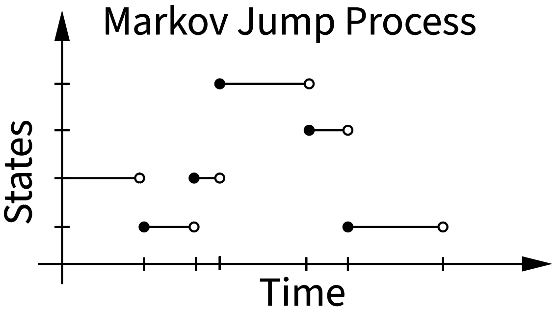
If you did some mathematics in French, the term cadlag should ring a bell which translates to ‘continue à droite, limite à gauche’ (right-continuous with left limits). You can observe the cadlag property of CTMC’s in the image where the empty circle is on the left side and the new state after a discrete jump is in the next state. Thus you can approach any point from the right, where the time index is defined in the ‘next’ state, but from the left you will see a jump. Said more simply: In case we jump at time $t$, the state at $t$ will be the ‘next’ state, not the previous state.

These jumps between states are stochastic and occur at stochastic times (check the x axis in the plot). The probability whether we do a jump is determined by the corresponding transition probability $p_{t+\Delta t | t}(y | x)$. If we were working with a discrete time Markov chain we would be done know since time would be discretized in $\Delta t$ segments anyway. But we’re dealing with continuous time so the discrete time transition probability doesn’t cut it. We’re interested in the transition rate.

The rate of a jump from state $x$ to state $y$ is the infinitissimal change in the transition probability $p_{t+\Delta t | t}(y|x)$ which denotes the probability of jumping from state $x$ to state $y$ at time $t$ for an infinitissimally small $\Delta t$: \(\begin{align} \lim_{\Delta t \rightarrow 0^+} p_{t + \Delta t | t}(y | x) = r_t(y|x) \end{align}\) Thus the rate $r_t(y|x)$ at a particular time $t$ denotes the instantaneous propensity / proclivity / tendency of moving from state $x$ to state $y$. Similarly, this is closely related to the Taylor expansion of the transition probability: \(\begin{align} p_{t + \Delta t | t}(y | x) &= \overbrace{p_{t|t}(y|x)}^{=\delta_{y,x}} + \lim_{\Delta t \rightarrow 0^+} p_{t + \Delta t | t}(y | x) \Delta t \\ &= \delta_{y,x} + r_t(y|x) \Delta t \end{align}\) where $\delta_{x,y}$ is the Kronecker delta.

There is actually a very nice extended derivation we can do to show the purpose and interactions of the rates $r_t(y|x)$ with the marginal probability distribution $p_t(x)$. The marginal probability $p_{t+\Delta t}(x)$ of state $x$ for a CTMC consists of all the movements from all other states $y$ into state $x$ and the probability of moving out of state $x$ to any other state $y$: \(\begin{align} p_{t+\Delta t}(x) &= p_{t}(x) - p_t(x) \overbrace{\sum_{y\neq x} p_{t+\Delta t| t}(y|x)}^{x \rightarrow y} + \underbrace{\sum_{y\neq x} p_t(y) p_{t+ \Delta t | t}(x | y)}_{y \rightarrow x} \\ &= p_{t}(x) \big( 1 - \sum_{y\neq x} (\delta_{x,y} + r_t(y|x) \Delta t) \big) + \sum_{y\neq x} p_t(y) (\delta_{y,x} + r_t(x|y) \Delta t) \end{align}\) Since $\delta_{x,y}$ always evaluates to zero as we only consider cases where $x\neq y$, we get \(\begin{align} p_{t+\Delta t}(x) &= p_{t}(x) \big( 1 - \sum_{y\neq x} (\overbrace{\delta_{x,y}}^{=0} + r_t(y|x) \Delta t) \big) + \sum_{y\neq x} p_t(y) (\overbrace{\delta_{y,x}}^{=0} + r_t(x|y) \Delta t) \\ &= p_{t}(x) \big( 1 - \sum_{y\neq x} r_t(y|x) \Delta t\big) + \sum_{y\neq x} p_t(y) r_t(x|y) \Delta t \\ \end{align}\) Rounding it off by pulling $p_t(x)$ to the right side and dividing by $\Delta t$, we get \(\begin{align} p_{t+\Delta t}(x) &= p_{t}(x) \big( 1 - \sum_{y\neq x} (\overbrace{\delta_{x,y}}^{=0} + r_t(y|x) \Delta t) \big) + \sum_{y\neq x} p_t(y) (\overbrace{\delta_{y,x}}^{=0} + r_t(x|y) \Delta t) \\ \frac{p_{t+\Delta t}(x) - p_t(x)}{\Delta t} &= - p_t(x) \sum_{y\neq x} r_t(y|x) + \sum_{y\neq x} p_t(y) r_t(x|y) \\ \dot{p}_{t}(x) &= - p_t(x) \sum_{y\neq x} r_t(y|x) + \sum_{y\neq x} p_t(y) r_t(x|y) \quad \leftarrow \text{master equation for CTMCs} \end{align}\)

Thus we have obtained a differential equation for our probabilities $p_t(x)$. The change in the probability of a single state $x$ is described by the current state $p_t( \cdot )$ and the rates $r_t( \cdot | \cdot)$ which can be understood as the dynamics of stochastic process which “move” probability between the states. The higher the rate $r_t(x|y)$, the more probable the process is to jump to the next state $x$ from state $y$. In terms of the marginal probability $p_t(x)$, this means there is a higher probability of being in the $x$ and thus the rate $r_t(x|y)$ “moves” more probability from state $y$ to state $x$.

More intuitively, we can simplify the above equation to just two states, for example $a$, $b$ and obtain \(\begin{align} \dot{p}_{t}(a) &= \underbrace{\overbrace{- r_t(b|a)}^{\text{outflow}} p_t(a)}_{\text{proportional outflow from a|}} \underbrace{\overbrace{+ r_t(a|b)}^{\text{inflow}} p_t(b)}_{\text{proportional inflow from b}} \\ \end{align}\)

The Ehrenfest Process

The Ehrenfest process is a very particular type of jump process (jump because we do discrete jumps between states). Namely it is a birth-death process which can only move to its immediate neighboring states. Check my previous blog post on CTMC’s for an in depth treatment.

The rates of the normal Ehrenfest process $E_S$ is \(\begin{align} \underbrace{r(x+1 | x) = \frac{1}{2}(S-x)}_{\text{birth rate}} \quad \quad \quad \underbrace{r(x-1| x) = \frac{x}{2}}_{\text{death rate}}. \end{align}\)

In a state space $x \in {0, \ldots, S}$ the birth and death rates are defined by linear functions in terms of the state. Thus, the birth rate is maximal when $x=0$ for which we have $r(x+1 | x) = \frac{1}{2}S$ and minimal when $x=S$ when its zero. Similarly, the death rate will be maximal when $x=S$ and minimal when $x=0$. The interesting connection arises when we observe the two rates in tandem. At $x=0$ only the birth rate will be non-negative such that we will do an increment step with absolute surety. Equally, at $x=S$, the birth rate will be zero and the we will make a decrement move with the death rate with absolute certainty. The result of this is that the Ehrenfest process is a birth-death process which is automatically confined to the state space $x \in \{0, \ldots, S\}$.

As a little thought experiment, one could think of what happens if we simulate such a process for a very long time. If the state increases too much, the death rate will overwhelm the birth rate and there will be a correction. Equally, if the state becomes too low, the birth rate will increase and the process will be pushed up again. From these two observations we can intuitively conclude that there has to exist an equilibrium distribution, probably in the center of the state space right around $S/2$.

The Scaled Ehrenfest Process

A very consequential insight made first in Sumita et al. was that there exists a very particular Ehrenfest process, which has properties which we’re familiar with even more.

We can shift ($-S/2$) and scale ($2/\sqrt{S}$) the Ehrenfest process to obtain the Scaled Ehrenfest Process, \(\begin{align} \tilde{E}_S(x) = \frac{2}{\sqrt{S}} \left( E_S - \frac{S}{2}\right). \end{align}\) with $x \in \{-\sqrt{S},-\sqrt{S} + \frac{2}{\sqrt{S}}, \ldots, \sqrt{S}\}$. Where previously the difference between states was a multiple of $\pm 1$, now the difference between states is just $\frac{2}{\sqrt{S}}$.

What are the rates of this scaled process if we play around with the state space by shifting and squeezing it?

We can express the scaled and shifted random variable as \(\begin{align} x' = \frac{2}{\sqrt{S}} ( x - \frac{S}{2}) \\ x = \frac{\sqrt{S}}{2} x' + \frac{S}{2} \end{align}\) and plug that right into the original rates of the unscaled Ehrenfest process \(\begin{align} r(x' + \frac{2}{\sqrt{S}}|x') &= \frac{1}{2}\left(S - \left(\frac{\sqrt{S}}{2} x' + \frac{S}{2}\right)\right) \\ &= \frac{1}{2}\left(\frac{S}{2} - \frac{\sqrt{S}}{2} x' \right)\\ &= \frac{1}{2}\left(\frac{\sqrt{S}\sqrt{S}}{2} - \frac{\sqrt{S}}{2} x' \right) \\ &= \frac{\sqrt{S}}{4}\left(\sqrt{S} - x' \right) \\ r(x' - \frac{2}{\sqrt{S}}|x') &= \frac{1}{2}\left(\frac{\sqrt{S}}{2} x' + \frac{S}{2}\right) \\ &= \frac{1}{2}\left(\frac{\sqrt{S}}{2} x' + \frac{\sqrt{S}\sqrt{S}}{2}\right) \\ &= \frac{\sqrt{S}}{4}\left(\sqrt{S} + x' \right) \end{align}\)

Now we can inspect the first and second jump moments which are analogous to the drift and diffusion coefficient estimation in continuous state space SDE’s \(\begin{align} b(x) &= \sum_{y\neq x} (y-x) r(y|x) \\ D(x) &= \sum_{y\neq x} (y-x) (y-x)^\top r(y|x) \end{align}\)

Whereas for the categorical Markov jump processes the sum would be quite long (in fact as long as the number of states minus the state itself), for a birth death process this reduces just to two summands since we can only make two possible moves in a state not on the boundary and a single move at the boundary.

For the scaled Ehrenfest process we obtain the following jump moments (remember that $(y-x) \in \{-\frac{2}{\sqrt{S}}, +\frac{2}{\sqrt{S}}\}$): \(\begin{align} b(x') &= \sum_{y'\neq x'} (y'-x') r(y'|x') \\ &= -\frac{2}{\sqrt{S}} \frac{\sqrt{S}}{4}\left(\sqrt{S} + x' \right) +\frac{2}{\sqrt{S}} \frac{\sqrt{S}}{4}\left(\sqrt{S} - x' \right) \\ &= \frac{2}{\sqrt{S}} \frac{\sqrt{S}}{4}\left(-\left(\sqrt{S} + x' \right) + \sqrt{S} - x' \right) \\ &= \frac{1}{2} \left(- 2x' \right) \\ &= -x' \\ D(x') &= \sum_{y'\neq x'} (y'-x') (y'-x')^\top r(y'|x') \\ &= \left(-\frac{2}{\sqrt{S}}\right)^2 \frac{\sqrt{S}}{4}\left(\sqrt{S} + x' \right) +\left(\frac{2}{\sqrt{S}}\right)^2 \frac{\sqrt{S}}{4}\left(\sqrt{S} - x' \right) \\ &= \frac{4}{S} \frac{\sqrt{S}}{4}\left(\sqrt{S} + x' \right) +\frac{4}{S} \frac{\sqrt{S}}{4}\left(\sqrt{S} - x' \right) \\ &= \frac{1}{\sqrt{S}} \left(\sqrt{S} + x' \right) +\frac{1}{\sqrt{S}}\left(\sqrt{S} - x' \right) \\ &= \frac{1}{\sqrt{S}} \left(\sqrt{S} + x' + \sqrt{S} - x' \right) \\ &= 2 \end{align}\)

Thus, in law, the scaled Ehrenfest process converges to a continuous state space stochastic process with the drift $-x$ and the diffusion $2$. This just so happens to identical to the Ornstein-Uhlenbeck process, $dX_t = -X_t dt + \sqrt{2} dW_t$. The OU process is used ubiquitously in variance preserving diffusion processes in generative diffusion models.

We can visualize this quite succinctly (shout out to my co-author Lorenz Richter) and have a look at the dynamics of the scaled Ehrenfest process with increasing state spaces. Down below are two Ornstein-Uhlenbeck processes starting from a Gaussian centered at $+1$ and $-1$ and converging towards their equilibrium distribution as time progresses to the right. We can see the convergence in law towards of the Ehrenfest process as we start to increase the state space $S$:

From this blog post we know that the analytical solution of the OU process $dX_t = - X_t dt + \sqrt{2} dW_t$ with zero mean is a time dependent Gaussian with mean and variance \(\begin{align} \mathbb{E}[X_t] &= e^{-t} X_0 \\ \mathbb{V}[X_t] &= 2(1-e^{-2t}) \\ & \downarrow \\ X_t &\sim \mathcal{N}(e^{-t} X_0, 2(1-e^{-2t})) \end{align}\) with the tractable solution of the forward process $p_{t|0}(x_t) = \mathcal{N}(e^{-t} X_0, 2(1-e^{-2t}))$.

That was the forward process but naturally in generative diffusion modelling we’re also interested in the time reversed stochastic process. For that we first have to derive the reverse time rates.

If we aim to revert a stochastic process in time, we have to make sure that in fact the forward evolution is exactly the same as the backward evolution. Otherwise, if one of the two directions behave differently, there quite literally not the same.

The necessary condition of a time reversal (also prominent in MCMC) is \(\begin{align} \lim_{\Delta t \rightarrow 0^+} p_{t-\Delta t |t}(y|x) p_t(x) &= \lim_{\Delta t \rightarrow 0^+}p_{t +\Delta t|t}(x|y) p_t(y) \\ r^-_t(y|x) p_t(x) &= r_t^+(x|y)p_t(y) \end{align}\) where (due to mathjax’s limited typesetting support) $r^-$ denotes the reverse-time/backward rate and $r^+$ the forward rate. The forward rate $r^+$ is usually provided through some sort of OU process with a tractable equilibrium distribution. The reverse rate $r^-$ is the thing of interest, since if we have the reverse rate we can actually revert the stochastic process and sample images from pure noise. Importantly, since the forward process is tractable, we can compute the analytical probability of a diffused sample $x_t$ from an data point $x_0$ (since the OU process is tractable).

A bit of algebra yields using the previously defined tractable conditional forward process $p_{t|0}(x_t|x_0)$ yields: \(\begin{align} r^-_t(y|x) &= \frac{p_t(y)}{p_t(x)} r_t(x | y) \\ &= \frac{\sum_{x_0} p_{t|0}(y|x_0) p_0(x_0)}{p_{t}(x)} r_t(x | y) \\ &= \sum_{x_0} \frac{ p_{t|0}(y|x_0)}{ p_t(x | x_0)} \frac{p_{t|0}(x | x_0) p_0(x_0)}{p_{t}(x)} r_t(x | y) \\ &= \sum_{x_0} \frac{ p_{t|0}(y|x_0)}{ p_{t|0}(x | x_0)} \ p_{0|t}(x_0 | x) r_t(x | y)\\ &= \mathbb{E}_{x_0 \sim \underbrace{p_{0|t}(x_0 | x)}_{\text{unknown}}} \underbrace{\left[ \frac{ p_{t|0}(y|x_0)}{ p_{t|0}(x | x_0)} \right]}_{\text{known}} \underbrace{r_t(x | y)}_{\text{known}}, \end{align}\)

If we examine the ratio, we know that $x$ and $y$ are only a $2/\sqrt{S}$ step apart from each other ($y=x \pm 2/\sqrt{S}$) for the scaled Ehrenfest process. Thus we can examine the ratio and rewrite it as \(\begin{align} \frac{ p_{t|0}(y|x_0)}{ p_{t|0}(x | x_0)} &=\frac{ p_{t|0}(x \pm \frac{2}{\sqrt{S}}|x_0)}{ p_{t|0}(x | x_0)} \end{align}\)

Now, we’re going to apply every physicists favourite tool and use a Taylor expansion on the nominator \(\begin{align} \frac{ p_{t|0}(y|x_0)}{ p_{t|0}(x | x_0)} &=\frac{ p_{t|0}(x \pm \frac{2}{\sqrt{S}}|x_0)}{ p_{t|0}(x | x_0)} \\ &=\frac{ p_{t|0}(x|x_0) \pm \frac{2}{\sqrt{S}}\nabla_x p_{t|0}(x|x_0) }{ p_{t|0}(x | x_0)} \\ &=1 \pm \frac{2}{\sqrt{S}} \underbrace{\frac{\nabla_x p_{t|0}(x|x_0) }{ p_{t|0}(x | x_0)}}_{\text{log derivative trick}} \\ &=1 \pm \frac{2}{\sqrt{S}} \nabla_x \log p_{t|0}(x | x_0) \end{align}\)

Oha, now suddenly the (conditional) score term has appeared in our Ehrenfest diffusion model. Coupled with the knowledge that in the large state space limit $S \rightarrow \infty$, we obtain a forward OU process as the marginal distribution of the scaled Ehrenfest process, we can substitute the obtained term back into the rates and get \(\begin{align} r^-_t(y|x) &= \mathbb{E}_{x_0 \sim p_{0|t}(x_0 | x)} \left[ \frac{ p_{t|0}(y|x_0)}{ p_{t|0}(x | x_0)} \right]r_t(x | y) \\ &= \mathbb{E}_{x_0 \sim p_{0|t}(x_0 | x)} \left[ 1 \pm \frac{2}{\sqrt{S}} \nabla_x \log p_{t|0}(x | x_0) \right]r_t(x | y)\\ &= \left( 1 \pm \frac{2}{\sqrt{S}} \mathbb{E}_{x_0 \sim p_{0|t}(x_0 | x)} \left[ \nabla_x \log p_{t|0}(x | x_0) \right] \right) r_t(x | y) \end{align}\) It turns out that the term \(\mathbb{E}_{x_0 \sim p_{0|t}(x_0 | x)} \left[ \nabla_x \log p_{t|0}(x | x_0) \right]\) is precisely the term that can be extracted from an score based generative diffusion model such as DDPM. Thus we can simulate a discrete state space samples with models and quantity obtained form their continuous counterparts.

For all the remaining extra stuff and math, read our paper here https://arxiv.org/pdf/2405.03549.