The Adjoint Method for Neural ODE's
Two perspectives on Memory Efficient Gradients
For my recent work, we started working on a custom made adjoint method to compute gradients for ODE’s with particular constraints. Since the 2019 paper at Neurips I was familiar with the problem that the adjoint method in neural ODE’s was trying to solve, yet I hadn’t really understood it in depth.
So for the implementation of our recent ideas I really had to dig into the adjoint method in order to implement it from scratch. Since I’m no Jeff Dean, I quickly found myself googling particular questions regarding the adjoint method. Yet, I found most expositions on the adjoint method somewhat clunky and cumbersome to understand. For that reason I’m going to add my two cents to this topic with this blog post.
The Setup & The Motivation
Fundamentally for neural ODE’s, we’re dealing with the model \(\begin{align} dx_t = f(x_t, t, \theta) \end{align}\) which we integrate with the initial condition $x_0$ to obtain a later value $x_T$, \(\begin{align} x_T &= x_0 + \int_{0}^T f(x_\tau, \tau, \theta) d\tau \\ &\approx x_0 + \sum_i f(x_{\tau_i}, \tau_i, \theta) \Delta \tau \quad \quad \quad \leftarrow \text{discrete approximation} \end{align}\) where we approximate the true solution with a discrete scheme which is known as the Euler integrator.
Then we compare our output $x_T$ (and optionally also our intermediate outputs $x_t$) with the target values $y_T$ \(\begin{align} \mathcal{L}(x_T, y_T) = ||x_T - y_T||^2 \end{align}\) which can be as simple as computing the MSE between prediction $x_T$ and target $y_T$.
One very important property of ODE’s is the Picard-Lindelöf Theorem (uniqueness theorem) which in our case states that the initial value problem which we solved in equation (2) has a unique solution. In practical terms this means that for a trajectory/solution $x_t$ through space and time, there exists a single trajectory from any initial condition $x_0$ to that particular $x_t$. Equally, for a given vector field characterized by $f(x, t, \theta)$ we can always recover the initial condition $x_0$ if we are given the tuple $(x_t, t)$ as we can simply integrate the vectorfield backwards until we reach $(x_0, 0)$.
As a counterfactual example, if the original vector field could for some reason randomly switch directions such that $dx_t = \pm f(x_t, t, \theta)$ the uniqueness property wouldn’t hold anymore. In this case, for a positive sign, we would still recover the original $x_0$ but if the function would randomly switch to a negative sign, we would integrate backwards to a different $x_0$. This, due to the stochastic switching, would be a stochastic differential equation.
Once we have our loss $\mathcal{L}$ we naturally want to compute the gradients $\partial \mathcal{L}/\partial \theta$ to update our parameters $\theta$ to minimize the loss $\mathcal{L}$.
What is the best way to to that?
The Autograd Approach
Fundamentally, we’re working with ODE’s here. Let’s investigate the gradient computation in these parameterized ODE’s and see if and how we can use the unique solution property of ODE’s for some gradient improvement.
Without loss of generality, we can stick with the Euler discretization to build up some intuition. Furthermore, we will only do three steps and use $x_3$ as our prediction to compare it to $y_3$, \(\begin{align} x_1 &= x_0 + f(x_0, 0, \theta) \Delta t \\ x_2 &= x_1 + f(x_1, 1, \theta) \Delta t \\ %= x_0 + f(x_0, 0, \theta) \Delta t + f(x_1, 1, \theta) \Delta t \\ x_3 &= x_2 + f(x_2, 2, \theta) \Delta t \\ %= x_0 + f(x_0, 0, \theta) \Delta t + f(x_1, 1, \theta) \Delta t + f(x_2, 2, \theta) \Delta t \end{align}\) A quick glance at the three equations above tells us that our parameters $\theta$ occur at every of the three time step. Consequentially, the total gradient $\frac{\partial \mathcal{L}}{\partial \theta}$ would consist of three additive terms, \(\begin{align} \frac{\partial \mathcal{L}}{\partial \theta} &= \sum_{t \in \{1,2,3\}} \frac{\mathcal{L}}{\partial x_t} \frac{\partial x_t}{\partial \theta} \\ &= \frac{\mathcal{L}}{\partial x_1} \frac{\partial x_1}{\partial \theta} + \frac{\mathcal{L}}{\partial x_2} \frac{\partial x_2}{\partial \theta} + \frac{\mathcal{L}}{\partial x_3} \frac{\partial x_3}{\partial \theta} \\ &= \frac{\mathcal{L}}{\partial x_3} \frac{\partial x_3}{\partial x_2} \frac{\partial x_2}{\partial x_1} \frac{\partial x_1}{\partial \theta} + \frac{\mathcal{L}}{\partial x_3} \frac{\partial x_3}{\partial x_2} \frac{\partial x_2}{\partial \theta} + \frac{\mathcal{L}}{\partial x_3} \frac{\partial x_3}{\partial \theta} \\ % &= \frac{\mathcal{L}}{\partial x_3} \sum_{t \leq 3} \prod_{t < t'} \frac{\partial x_{t'+1}}{\partial x_{t'}} \frac{\partial x_{t'}}{\partial \theta} \end{align}\)
Looking at the equation above, your reverse-autograd/vector-jacobian product senses should start to tingle. The calculation of $x_3$ moved ‘forward’ in time ($x_1 \rightarrow x_2 \rightarrow x_3$) whereas the gradients move in ‘reverse’ time through the computation (\(\frac{\mathcal{L}}{\partial x_3} \frac{\partial x_3}{\partial x_2} \frac{\partial x_2}{\partial x_1} \frac{\partial x_1}{\partial \theta}\) and thus $x_1 \leftarrow x_2 \leftarrow x_3$ is a good example).
The partial derivative $\frac{\partial x_{t+1}}{\partial x_t}$ keeps occurring a lot of times, particularly if we consider time series with more than our puny three steps. So let’s examine this derivative in more detail and let’s take $\frac{\partial x_3}{\partial x_2}$ as an example: \(\begin{align} \frac{\partial x_3}{\partial x_2} &= \frac{\partial \ x_2 + f(x_2, 2, \theta) \Delta t}{\partial x_2} \\ &= 1 + \frac{\partial f(x_2, 2, \theta)}{\partial x_2}\Delta t \end{align}\)
Generalizing the time indices from this particular example, we get \(\begin{align} \underbrace{\frac{\partial x_t}{\partial x_{t-1}}}_{\text{quantity}} = 1 + \underbrace{\frac{\partial f(x_{t-1}, t-1, \theta)}{\partial x_{t-1}}}_{\text{change}} \underbrace{\Delta t}_{\text{time step}} \end{align}\) which seems to look like a somewhat crude ODE itself which was solved with a weird form of the Euler integrator with an initial condition of $1$. The change in the gradient as we move backwards through time seems to be some function we can evaluate (the derivative just being an operator) multiplied by some time differential.
More consequentially, we can also have a closer look at $x_{t-1}$. From earlier, we have the relation \(\begin{align} x_t = x_{t-1} + f(x_{t-1}, t-1, \theta) \Delta t \end{align}\) which describes how we can obtain a later part of the solution $x_t$ from the earlier solution $x_{t-1}$. Are we allowed to do that? Yes, because the Picard-Linedlöf/Cauchy-Lipschitz/Uniqueness Theorem tells us that for any tuple $(x_t, t)$ in a smooth vector field there is a unique trajectory. The time reversibility of ODE’s allows us to equally apply a reverse time (discrete) solution by using \(\begin{align} x_{t-1} = x_{t} - f(x_t, t, \theta) \Delta t. \end{align}\)
This implies that we can calculate the gradient $\frac{\partial x_t}{x_{t-1}}$ purely from the current state $x_t$, \(\begin{align} \frac{\partial x_t}{\partial x_{t-1}} = 1 + \frac{\partial f(x_{t-1}, t-1, \theta)}{\partial \color{blue}{x_{t-1}}} \ \Delta t \ \Bigg|_{\color{blue}{x_{t-1}} = x_{t} - f(x_t, t, \theta) \Delta t} \end{align}\)
This is kind of big news in terms of memory requirements when calculating gradients.
You see, in reverse mode differentiation, we need to store the data that we generate during the forward pass to compute gradients during the backward pass.
A very simple but illuminating example is computing gradients for an affine, scalar function
\(\begin{align}
y &= w \cdot x \\
\frac{\partial y}{\partial x} &= w \\
\frac{\partial y}{\partial w} &= x
\end{align}\)
from which we can see that we need to store the input data $x$ in order to calculate gradients with respect to our parameter $w$.
In PyTorch, this is implemented within autograd (link here) with the autograd.Function and the corresponding ctx keyword which acts as a storage unit to save all relevant data values for the computation of the gradients.
The time-reversibility (and the uniqueness theorem) of our ODE allows us to not actually having to store the data, but instead recompute it.
We can take the gradient \(\frac{\mathcal{L}}{\partial x_3} \frac{\partial x_3}{\partial x_2} \frac{\partial x_2}{\partial x_1} \frac{\partial x_1}{\partial \theta}\) as an example.
Reverse-mode autodifferentiation will compute vector-Jacobian products,
\(\begin{align}
\frac{\partial \mathcal{L}}{\partial x_1}
&= \underbrace{\overbrace{\frac{\mathcal{L}}{\partial x_3}}^{\text{vector} \ g_3} \ \overbrace{\frac{\partial x_3}{\partial x_2}}^{\text{Jacobian}\ J}}_{g_2 = g_3^T J} \frac{\partial x_2}{\partial x_1} \frac{\partial x_1}{\partial \theta} \\
&= \underbrace{g_2 \overbrace{\frac{\partial x_2}{\partial x_1}}^{\text{Jacobian} \ J}}_{g_1 = g_2^T J} \frac{\partial x_1}{\partial \theta} \\
&= \underbrace{g_1 \overbrace{\frac{\partial x_1}{\partial \theta}}^{\text{Jacobian} \ J}}_{g = g_1^T J} \\
\end{align}\)
and at each Jacobian $\frac{\partial x_t}{x_{t-1}}$ instead of storing the data in ctx of PyTorchs autograd functionality, we simply recompute $x_{t-1}$ and construct the Jacobian (to be used in the efficient vector-Jacobian product) as
\(\begin{align}
\frac{\partial x_t}{\partial x_{t-1}} = 1+ \frac{\partial f(x_{t-1}, t-1, \theta)}{\partial x_{t-1}} \ \Delta t \ \Bigg|_{x_{t-1} = x_{t} - f(x_t, t, \theta) \Delta t}
\end{align}\)
Here, the $1$ should also become more clear when we embed it into a chain rule \(\begin{align} \underbrace{\frac{\partial x_{t+1}}{\partial x_t}}_{\text{incoming gradient}} \frac{\partial x_t}{\partial x_{t-1}} = \underbrace{\frac{\partial x_{t+1}}{\partial x_t}}_{\text{incoming gradient}} \underbrace{\left(1+ \frac{\partial f(x_{t-1}, t-1, \theta)}{\partial x_{t-1}} \ \Delta t \ \Bigg|_{x_{t-1} = x_{t} - f(x_t, t, \theta) \Delta t} \right)}_{\text{multiplicative update}} \end{align}\) where we multiply the ‘incoming gradient’ from a deeper part of the computational graph with a multiplicative update. The Jacobian slightly updates the otherwise constant multiplicative update factor of $1$. The finer we choose $\Delta t$ the finer the update to the gradient will be which sounds very ODE-like.
I would like to highlight that we’re actually computing the vector-Jacobian product $g^T J$, which is PyTorch’s “native” gradient computation. Computing the Jacobian for a function $f: \mathbb{R}^{100} \rightarrow \mathbb{R}^{50}$ would require us to do $100 \times 50 = 5.000$ individual gradient evaluations. The Jacobian matrix measure the sensitivity of each output to a particular input independent of all other inputs. Mathematically, this forces us to compute every input-output combination manually, as a parallel evaluation of two or more Jacobian entries would “mix gradients” and thus be wrong.
But we’re not really interested in the complete data-agnostic Jacobian matrix. We already used (conditioned on) data such that our gradient computation (and thus the Jacobian) is in fact a directional derivative. We’re not asking: “For any data, what is the gradient?” but rather “What’s the gradient on this particular loss surface that has been determined by the data?”. Essentially, whereas the Jacobian would measure the independent sensitivity of an input-output pair, with the forward pass we already sort of ‘threw the baby out of the window with bath water’ as the forward pass already determined the interaction of the inputs and outputs (it’s not data agnostic anymore and i.e. determined by a convolution layer). The use of data already fixed the input-output interaction and the gradient now flows along the path charted by the data in the forward pass. This allows us to instead compute vector-Jacobian products which essentially traverses the entire computational graph in reverse order.
Thus during the backward pass we only need the current gradient $g_t$ (often referred to as the adjoint $a(t)$ or $\lambda(t)$ in the literature) in between the function evaluations and the current state $x_t$ to compute all relevant gradients.
Imagine that you have a GPU with 40GB of memory and each model evaluation consumes 1GB through the activation storage. Thus you’re hamstrung to only 40 evaluations before your GPU is full. By using the adjoint method you can scale up your batch size to $40\times$ or use a much larger network since you ever only hold a single evaluation $f(x_t, t, \theta)$ in memory when doing the backward pass.
The Lagrangian Derivation
The approach above was based on an Euler discretization scheme for ODE’s. We saw how we could use the unique solution/time reversibility property to actually circumvent the explicit storing of the entire computational graph.
Yet, of all the solvers out there for ODE’s, Euler is by far the simplest … but also the worst. So in order to move away from the simple time discretization of Euler, we will have to go fully continuous.
Above was a very pragmatic way to look at the memory efficient adjoint gradient computation. In the second perspective we will take the math-y road and show how the adjoint quantity can be derived mathematically. This will allow us to write down a general gradient ODE for which we can use more sophisticated solvers beyond the Euler scheme.
As before, we consider the differential equation \(\begin{align} dx_t = f(x_t, t, \theta) \end{align}\) with a cost functional $J$ and a scalar loss $\mathcal{L}$ and a final loss $\mathcal{F}$ \(\begin{align} J(x,\theta) = \int_0^T \mathcal{L}(x_t, t, \theta) dt + \mathcal{F}(x_T) \end{align}\)
To minimize $J$ with respect to the parameters $\theta$ we need to compute the gradient $\frac{\partial J}{\partial \theta}$. But alas, $\theta$ also influences $x_t$ since it occurs in the original differential equation.
Since the dynamics pose a constraint that we have to fulfill at all times, we will add it as a time-dependent Lagrange multiplier $\lambda_t$, \(\begin{align} J_\lambda(x,\theta) = \int_0^T \mathcal{L}(x_t, t, \theta) dt + \mathcal{F}(x_T) + \int_0^T \lambda^\top_t \left( dx_t - f(x_t, t, \theta) \right) dt. \end{align}\)
The Lagrange multiplier $\lambda_t$ has the same dimensionality as $x_t$ … and just like the gradient $\frac{\partial x_{t+1}}{\partial x_t}$ … coincidence, I think not!
Next, we assume that a small perturbation in $x_t$ and $\theta$ influence the total perturbation in $J$ \(\begin{align} \delta J(x, \theta) = & \int_0^T \frac{\partial \mathcal{L}(x_t, t, \theta)}{\partial x_t} \ \color{red}{\delta x_t} \ + \frac{\partial \mathcal{L}(x_t, t, \theta)}{\partial \theta} \ \color{red}{\delta \theta} dt + \frac{\partial \mathcal{F}(x_T)}{\partial x_T} \color{red}{\delta x_T} \\ &+ \int_0^T \lambda^\top_t \left( \color{red}{\delta dx_t} - \frac{f(x_t, t, \theta)}{\partial x_t} \ \color{red}{\delta x_t} \ - \frac{f(x_t, t, \theta)}{\partial \theta} \ \color{red}{\delta \theta} \right) dt. \end{align}\)
The cost functional $J$ has two inputs $x$ and $\theta$ which also interact through $f$. One can intuit about it as $J$ having two degrees of freedom. We can wiggle a bit in the $x$ direction and $J$ would change. Or we can wiggle a bit in $\theta$ and $J$ would also change. Finally, we can wiggle in both $\theta$ and $x$ and then $J$ would change as well.
Unfortunately, this has variations in all degrees of freedom $\delta x_t$, $\delta \theta$, $\delta dx_t$ and even $\delta x_T$. Also, we still have the annoying time derivative $dx_t = \dot{x}_t$.
So far the perturbation $\delta J(x, \theta)$ still consists of both the perturbations in $x$ and $\theta$. But in machine learning, $x$ is the provided data and we’re really want to only quantify the perturbation in $\theta$. That perturbation in $\theta$ is precisely the gradient we need for gradient based optimization, as it quite literally encodes how much $J$ would change if we perturbed $\theta$ a bit.
Until know we haven’t made zero assumption about what the Lagrangian actually looks like. The idea of the adjoint method is to choose $\lambda_t$ in just such a way, that it completely eliminates the $\delta x$ perturbation from the total loss perturbation $\delta J$ such that we’re left with the parameter perturbation $\delta \theta$ which is our gradient.
But in the perturbed Lagrangian, there is still the perturbed time derivative $\delta dx_t = \delta \dot{x}_t$ which is unpleasant to work with, respectively we don’t even know what it might be. Could we maybe transform the perturbation in the time derivative $\delta dx_t$ into a perturbation in ‘just’ space $\delta x_t$? Here, integration by parts comes to the rescue! Namely, \(\begin{align} \int_0^T \lambda_t^\top \delta \color{red}{dx_t} dt = [\lambda_t^\top \delta x_t]_0^T - \int_0^T \color{red}{d\lambda_t}^\top \delta x_t dt \end{align}\) where we shifted the time derivative in $dx_t$ to the time derivative in $d\lambda_t$.
The integration by parts term further simplifies when we consider that we can’t perturb the initial condition $x_0$ as that is hard coded as data. \(\begin{align} \int_0^T \lambda_t^\top \delta dx_t dt &= [\lambda_t^\top \delta x_t]_0^T - \int_0^T d\lambda_t^\top \delta x_t dt \\ &= \lambda_T^\top \delta x_T - \lambda_0^\top \underbrace{\delta x_0}_{\color{red}{=0}} - \int_0^T d\lambda_t^\top \delta x_t dt \\ &= \lambda_T^\top \delta x_T - \int_0^T d\lambda_t^\top \delta x_t dt \end{align}\)
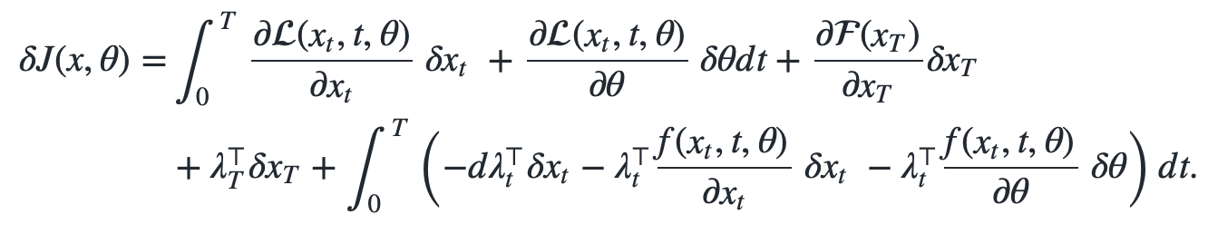
Thus our adapted perturbed functional loss now reads \(\begin{align} \delta J(x, \theta) = & \int_0^T \frac{\partial \mathcal{L}(x_t, t, \theta)}{\partial x_t } \ \delta x_t \ + \frac{\partial \mathcal{L}(x_t, t, \theta)}{\partial \theta} \ \delta \theta dt + \frac{\partial \mathcal{F}(x_T)}{\partial x_T} \delta x_T \\ &+ \lambda_T^\top \delta x_T + \int_0^T \left( -d\lambda_t^\top \delta x_t - \lambda_t^\top \frac{f(x_t, t, \theta)}{\partial x_t} \ \delta x_t \ - \lambda_t^\top \frac{f(x_t, t, \theta)}{\partial \theta} \ \delta \theta \right) dt. \end{align}\)
We can now rearrange the terms to make the Lagrangian $\lambda_t$ cancel out all the contributions of the space perturbations $\delta x_t$, \(\begin{align} \delta J(x, \theta) = & \quad \int_0^T \frac{\partial \mathcal{L}(x_t, t, \theta)}{\partial x_t } \ \delta x_t \ + \frac{\partial \mathcal{L}(x_t, t, \theta)}{\partial \theta} \ \delta \theta dt \\ & + \int_0^T -d\lambda_t^\top \delta x_t - \lambda_t^\top \frac{f(x_t, t, \theta)}{\partial x_t} \ \delta x_t \ - \lambda_t^\top \frac{f(x_t, t, \theta)}{\partial \theta} \ \delta \theta dt \\ & + \lambda_T^\top \delta x_T + \frac{\partial \mathcal{F}(x_T)}{\partial x_T} \delta x_T \\ = & \quad \int_0^T \underbrace{\frac{\partial \mathcal{L}(x_t, t, \theta)}{\partial x_t }}_{\color{red}{(1)}} \ \delta x_t \ + \frac{\partial \mathcal{L}(x_t, t, \theta)}{\partial \theta} \ \delta \theta dt \\ & + \int_0^T \underbrace{-\left( d\lambda_t^\top + \lambda_t^\top \frac{f(x_t, t, \theta)}{\partial x_t} \right)}_{\color{red}{(1)}} \ \delta x_t \ - \lambda_t^\top \frac{f(x_t, t, \theta)}{\partial \theta} \ \delta \theta dt \\ & \underbrace{+ \lambda_T^\top \delta x_T}_{\color{green}{(3)}} + \underbrace{\frac{\partial \mathcal{F}(x_T)}{\partial x_T} \delta x_T}_{\color{green}{(3)}} \end{align}\)
Now we can choose $\lambda_t$ in the following way: \(\begin{align} \color{green}{(3)}: \lambda_T^\top &= - \frac{\partial \mathcal{F}(x_T)}{\partial x_T} \\ \color{red}{(1)}: d\lambda_t^T &= \frac{\partial \mathcal{L}(x_t, t, \theta)}{\partial x_t } - \lambda_t^\top \frac{f(x_t, t, \theta)}{\partial x_t} \end{align}\)
The two equations above form the basis of the adjoint ODE where we formulated the terminal condition $\lambda_T^\top$ for the reverse ODE as well as the dynamics $d\lambda_t^\top$.
Since we’re solving an ODE, this also explains the $1 + \text{Jacobian} \ \Delta t$ from the autograd approach. Solving the adjoint state with the Euler integrator would correspond to \(\lambda_{t-1} = \lambda_t - \lambda_t \frac{\partial f(x_t, t, \theta)}{\partial x_t} \Delta t = \lambda_t \left( 1 - \frac{\partial f(x_t, t, \theta)}{\partial x_t} \Delta t \right)\) which is our Euler gradient integration from the autograd but with negative integration sign, since we’re going backwards in time.
Our current code base is under active development and subject to public restrictions so I’ll use the torchdiffeq library to highlight some heavily condensed code (code link):
def augmented_dynamics(t, y_aug):
                x_t = y_aug[1] # state
                adj_x_t = x_t_aug[2] # adjoint/continuous grad/lambda_t

                with torch.enable_grad():
                    x_t = x_t.detach().requires_grad_(True) # make x_t
                    '''Evaluate dx_t = f(x_t, t, θ) for state recomputation
                        x_{t-1} = x_t - f(x_t, t, θ) dt
                    '''
                    func_eval = func(t if t_requires_grad else t_, x_t)

                    '''Derive for
                        - state ∂f(x_t, t, θ) / ∂ x_t
                        - paramters ∂f(x_t, t, θ) / ∂ θ
                      in a single call
                      The adjoint adj_x_t is used as the gradient
                      that we backprop through the function
                    '''
                    vjp_x_t, *vjp_params = torch.autograd.grad(
                        output=func_eval,
                        input=(x_t) + adjoint_params,
                        output_gradient=-adj_x_t,
                        allow_unused=True, retain_graph=True
                    )
                '''
                func_eval: dx_t used in reverse_time integration -dx_t
                vjp_x_t: adjoint gradient propagated backward in time
                vjp_params: accumulate gradients in parameters on the fly
                '''
                return (func_eval, vjp_x_t, *vjp_params)
Comparing this to our ‘autograd engineering’ solution we can see that the adjoint $\lambda_t$ corresponds to our gradient vector $g$ and the extra minus sign stems from the time direction, which we didn’t consider in the ‘autograd engineering’ approach.
Remember how we used to go through the chain rule from the back during the autograd backpropagation? Intuitively the gradient $g_t$ that we propagated through the evaluations is a discrete time version of the continuous true gradient/adjoint $\lambda_t$: \(\begin{align} & \text{Discrete Euler/Autograd} & \text{Adjoint/Continuous Gradient} \\ \frac{\partial \mathcal{L}}{\partial x_1} &= \underbrace{\overbrace{\frac{\mathcal{L}}{\partial x_3}}^{\text{vector} \ g_3} \ \overbrace{\frac{\partial x_3}{\partial x_2}}^{\text{Jacobian}\ J}}_{g_2 = g_3^T J} \frac{\partial x_2}{\partial x_1} \frac{\partial x_1}{\partial \theta} & \rightarrow \lambda_3^\top \frac{\partial x_3}{\partial x_2}=\lambda_2\\ &= \underbrace{g_2 \overbrace{\frac{\partial x_2}{\partial x_1}}^{\text{Jacobian} \ J}}_{g_1 = g_2^T J} \frac{\partial x_1}{\partial \theta} & \rightarrow \lambda_2^\top \frac{\partial x_2}{\partial x_1} = \lambda_1 \\ &= \underbrace{g_1 \overbrace{\frac{\partial x_1}{\partial \theta}}^{\text{Jacobian} \ J}}_{g = g_1^T J} & \rightarrow \lambda_1^\top \frac{\partial x_1}{\partial x_\theta} = \frac{\partial \mathcal{L}}{\partial \theta}\\ \end{align}\)
Once we solved the adjoint ODE $\lambda_t$ for all time steps $t$, we can simply use it as the vector in the vector-Jacobian product $\lambda^\top_t \frac{\partial f(x_t, t,\theta)}{\partial \theta}$ to compute the parameter gradients. Thus again, the adjoint $\lambda_t$ is so to say an instantaneous gradient surrogate as we used it in the classic time-discretized autograd vector-Jacobian $g^T J$, so $g = \text{TimeDiscretize}(\lambda_t)$.