Solving (Some) SDEs
Geometric Brownian Motion & Ornstein-Uhlenbeck Process
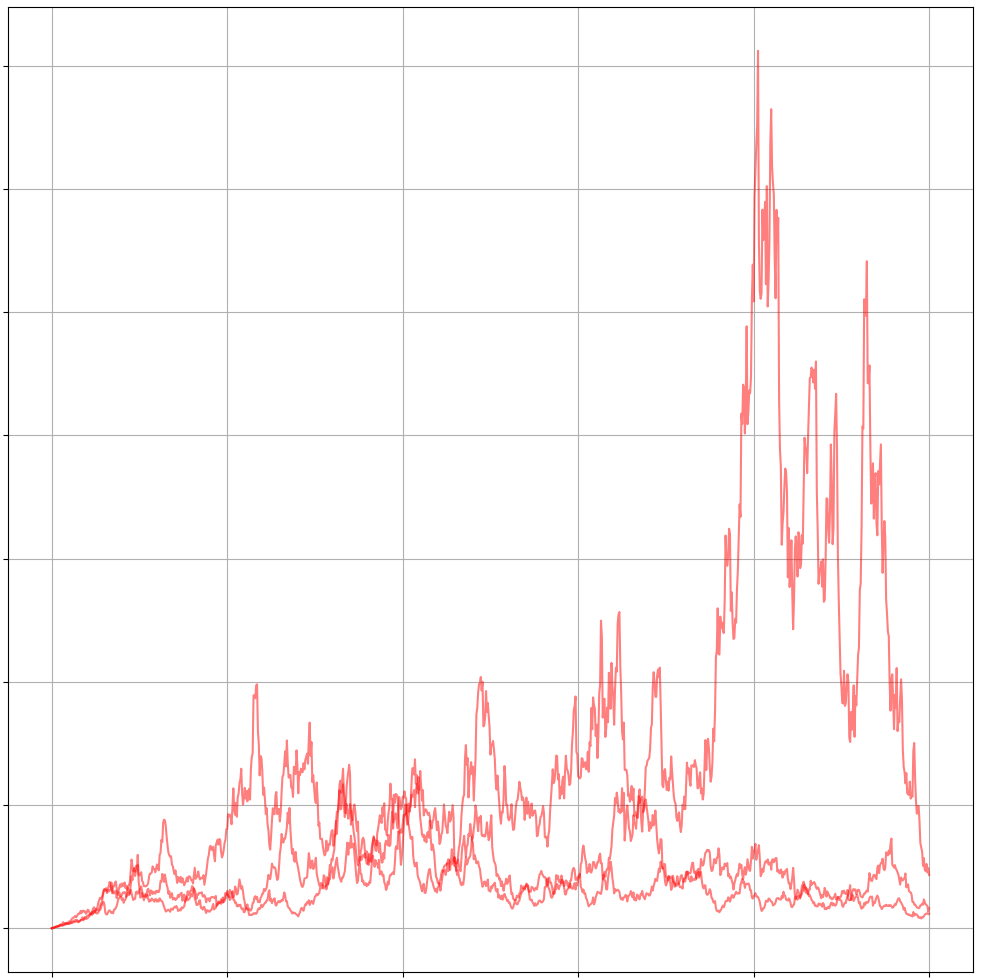
Geometric Brownian Motion
Brownian motion can have both positive and negative values as long as its mean is centered around zero and the distribution over time follows the characteristics of the Wiener process. Yet certain quantities can only have positive values such as stocks.
In order to accommodate the specific requirements of such quantities we can work with geometric Brownian motion, \(\begin{align} dS_t &= \mu_t S_t dt + \sigma_t S_t dW_t \\ \frac{dS_t}{S_t} &= \mu_t dt + \sigma_t dW_t \end{align}\) which has the nice property that as $S_t$ approaches zero, so does the change. This effectively limits $S_t$ to positive values, $S_t \geq 0$.
The question is as so often with differential equation, whether there exists an analytic solution. In order to show this analytic solution we will examine the quantity $dS_t/ S_t$ and apply the stochastic version of the log-derivative trick. The quantity $dS_t/S_t$ has a striking familiarity to \(\begin{align} \frac{\partial \ln S(x)}{\partial x} = \frac{1}{S(x)} \frac{\partial S(x)}{\partial x} \end{align}\) But since we are working with stochastic processes, we can’t apply regular calculus to derive such a stochastic process but use Ito’s lemma instead: \(\begin{align} d \ln S_t &= \underbrace{\frac{\partial \ln S_t}{\partial t}}_{=0} dt + \frac{\partial \ln S_t}{\partial S_t} dS_t + \frac{1}{2} \frac{\partial^2 \ln S_t}{\partial S_t^2} dS_t^2 \\ &= \frac{dS_t}{S_t} - \frac{1}{2} \frac{1}{S_t^2} (\mu_t S_t + \sigma_t S_t dW_t)^2 \\ &= \frac{dS_t}{S_t} - \frac{1}{2} \frac{1}{S_t^2} (\mu_t S_t dt + \sigma_t S_t dW_t)^2 \\ &= \frac{dS_t}{S_t} - \frac{1}{2} \frac{1}{S_t^2} (\mu_t^2 S_t^2 \underbrace{dt^2}_{\rightarrow 0} + 2 \mu_t S_t \underbrace{dt dW_t}_{\rightarrow 0} + \sigma_t^2 S_t^2 \underbrace{dW_t^2}_{=dt}) \\ &= \frac{dS_t}{S_t} - \frac{1}{2} \sigma_t^2 dt \\ \frac{dS_t}{S_t} &= d \ln S_t + \frac{1}{2} \sigma_t^2 dt \end{align}\) Since $\ln S_t$ does not have $t$ as an argument, the first term evaluates to zero. Plugging our alternative definition of \(\frac{dS_t}{S_t}\) into the original SDE and integrating it we obtain: \(\begin{align} d \ln S_t + \frac{1}{2} \sigma^2 dt &= \mu_t dt + \sigma_t dW_t \\ \int_0^t d \ln S_s &= \int_0^t \mu_s ds + - \int_0^t \frac{1}{2} \sigma_s^2 ds + \int_0^t \sigma_s dW_s \\ \ln S_t - \ln S_0 &= \mu_t t - \frac{1}{2} \sigma_t^2 t + \sigma_t W_t \\ \ln \frac{S_t}{S_0} &= \mu_t t - \frac{1}{2} \sigma_t^2 t + \sigma_t W_t \\ S_t &= S_0 \ e^{\mu_t t - \frac{1}{2} \sigma_t^2 t + \sigma_t W_t} \\ \end{align}\)
Ornstein-Uhlenbeck Process
The Ornstein-Uhlenbeck (OU) process is a SDE that exhibits mean reversion and momentum properties. Mathematically it is defined as: \(\begin{align} dX_t = \theta(\mu - X_t)dt + \sigma dW_t \end{align}\) where $\theta$ is the momentum parameter that makes the OU process undulate around the mean. The mean parameter $\mu$ sets the value around which the OU process moves in somewhat smooth arcs. Visually it looks like this:
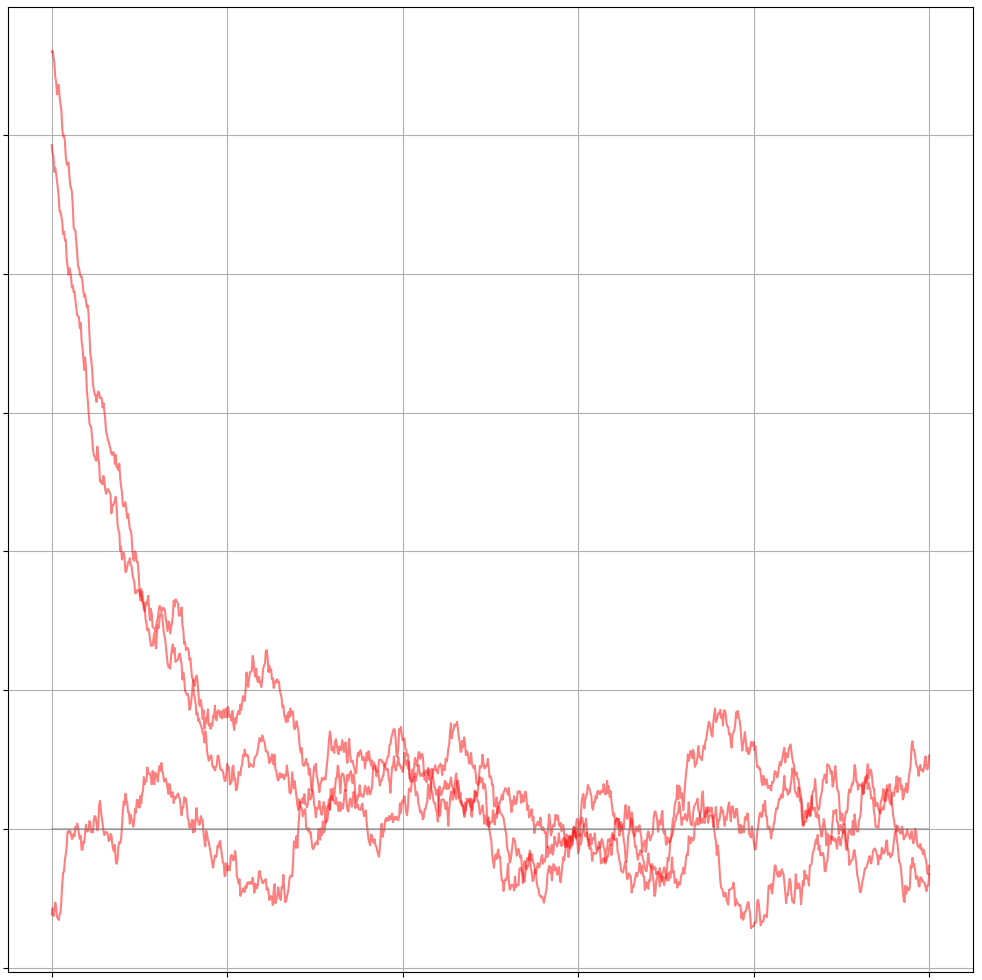
where we can see that even though two of the three sample paths start far away from the mean, they quickly converge to a region around the mean. Once in the vicinity of the mean they move about it in arcs through the momentum factor.
The first time I heard of the OU process was in a reinforcement learning paper where it was used to force an agent to repeat the same action a couple of times through the momentum property.
First, let’s try to clean up the notation to something more succinct and define a new random variable $Y_t$: \(\begin{align} Y_t = X_t - \mu \end{align}\) We can easily compute the infinitesimal differential $dY_t$ of $Y_t$ via: \(\begin{align} dY_t &= dX_t \\ &= \theta(\mu - X_t)dt + \sigma dW_t \\ &= - \theta \underbrace{(X_t - \mu)}_{Y_t}dt + \sigma dW_t \\ &= - \theta Y_tdt + \sigma dW_t \\ \end{align}\) The next step is to recognize that we are equating the derivative of a random variable with itself. We’ll abuse the mathematical notation for a brief period to make the point more clear: \(\begin{align} dY_t & \propto \theta Y_t dt \\ \frac{dY_t}{dt} &\propto \theta Y_t \Leftrightarrow \frac{d e^{ax}}{dx} = ae^x \end{align}\) The proportional equation above has a striking similarity to the derivative of a scaled exponential $e^{ax}$. In our case the derivative is not with respect to $x$ but to $t$. To solidify this intuition let’s define another random variable $Z_t$ as a function of $Y_t$: \(\begin{align} Z_t &= f(t, \theta, Y_t) \\ &= e^{\theta t} Y_t \end{align}\) The question naturally arises how $Z_T$ behaves in the infinitesimal differential $dZ_t$. But since $Z_t$ is a function of a stochastic process we will have to apply Ito’s lemma in order to compute the differential. Since $Z_t = f(t, \theta, Y_t)$ is linear in $Y_t$, we will deal with a simplified version of Ito’s lemma because the second derivative of a linear function is zero: \(\begin{align} df(t, \theta, Y_t) &= \partial_t \ f(t, \theta, Y_t) dt + \partial_{Y_t} \ f(t, \theta, Y_t) dY_t + \frac{1}{2} \overbrace{\partial_{Y_t}^2 \ f(t, \theta, Y_t)}^{=0} dY_t^2 \\ &=\partial_t \ f(t, \theta, Y_t) dt + \partial_{Y_t} \ f(t, \theta, Y_t) dY_t \end{align}\) Applying the simplified Ito’s lemma to our equation at hand yields: \(\begin{align} dZ_t &= \partial_{t} \left[e^{\theta t}Y_t \right] dt + \partial_{Y_t} \left[e^{\theta t}Y_t \right] dY_t \\ &= \theta e^{\theta t}Y_t dt + e^{\theta t} dY_t \\ &= \theta e^{\theta t}Y_t dt + e^{ \theta t}\left(-\theta Y_t dt + \sigma dW_t \right) \\ &= e^{\theta t} \sigma dW_t \end{align}\) This can be easily solved via \(\begin{align} Z_T &= Z_S + \int_{S}^T dZ_t \\ &= Z_S + \sigma \int_{S}^T e^{\theta t} dW_t \end{align}\) where $S$ is the start of the integration through time. Now that we found a solution to the random variable $Z_t$ it is time to go back through the substitutions to find the solution to $X_t$. In order to achieve that we first reverse the exponential component in the relationship between $Y_t$ and $Z_t$. \(\begin{align} Y_t &= e^{-\theta t}Z_t \\ Y_T &= e^{-\theta T} Z_T \\ &= e^{-\theta T}(Z_S + \sigma \int_{S}^T e^{\theta t} dW_t) \\ &=e^{-\theta T}(e^{kS} Y_S + \sigma \int_{S}^T e^{\theta t} dW_t) \\ &=e^{-\theta(T-S)} Y_S + \sigma e^{-\theta T} \int_{S}^T e^{\theta t} dW_t \\ &=e^{-\theta(T-S)} Y_S + \sigma \int_{S}^T e^{\theta(t-T)} dW_t \\ \end{align}\) Finally plugging $Y_t =X_t -\mu$ back in yields: \(\begin{align} Y_T &=e^{-\theta(T-S)} Y_S + \sigma \int_{S}^T e^{\theta(t-T)} dW_t \\ X_T - \mu &=e^{-\theta(T-S)} (X_S - \mu) + \sigma \int_{S}^T e^{\theta(t-T)} dW_t \\ X_T &= \mu + e^{-\theta(T-S)} (X_S - \mu) + \sigma \int_{S}^T e^{\theta(t-T)} dW_t \\ \end{align}\) Starting from $S=0$ we obtain \(\begin{align} X_T = \mu + e^{-\theta T}(X_0 - \mu) + \sigma \int_{S=0}^T e^{-\theta (T-t)} dW_t \end{align}\) In fact the Ornstein-Uhlenbeck process is one of the few stochastic processes that has a stationary distribution under the assumption of a Normal initial value. In order to show that we can compute the mean and variance of the process and then evaluate it in infinity with the limit of $\lim t\rightarrow 0$: \(\begin{align} \mathbb{E} \left[ X_t \right] &= \mathbb{E} \left[ \mu + e^{-\theta t}(X_0 - \mu) + \sigma \int_{s=0}^t e^{-\theta (t-s)} dW_s\right] \\ &= \mu + e^{-\theta t}(X_0 - \mu) + \underbrace{\mathbb{E} \left[ \sigma \int_{s=0}^t e^{-\theta (t-s)} dW_s\right]}_{\text{Wiener process} \rightarrow \mathbb{E}[W_t]=0} \\ &= \mu + e^{-\theta t}(X_0 - \mu) \end{align}\) and \(\begin{align} \mathbb{V} \left[ X_t \right] &= \mathbb{E} \left[ \left( X_t - \mathbb{E}[X_t] \right)^2 \right] \\ &= \mathbb{E} \Bigg[ \Big( \underbrace{\mu + e^{-\theta t}(X_0 - \mu)}_{=\mathbb{E}[X_t]} + \sigma \int_{s=0}^t e^{-\theta (t-s)} dW_s - \mathbb{E}[X_t] \Big)^2 \Bigg] \\ &= \mathbb{E} \left[ \left(\sigma \int_{s=0}^t e^{-\theta (t-s)} dW_s \right)^2 \right] \quad \leftarrow \text{Ito Isometry} \\ &= \sigma^2 \int_{s=0}^t e^{-2\theta (t-s)} ds \\ &= \sigma^2 \left[ \frac{1}{2\theta} e^{-2\theta (t-s)} \right]_{s=0}^t \\ &= \frac{\sigma^2}{2\theta} (e^{-2\theta*0} - e^{-2\theta t}) \\ &= \frac{\sigma^2}{2\theta} (1 - e^{-2\theta t}) \end{align}\) Applying the limit $\lim t \rightarrow \infty$ allows us to recover the stationary distribution: \(\begin{align} \lim_{t\rightarrow 0} \mathbb{E} \left[X_t\right] &= \lim_{t\rightarrow 0} \mu + \underbrace{e^{-\theta t}}_{=0}(X_0 - \mu) \\ &= \mu \\ \lim_{t\rightarrow 0} \mathbb{V}\left[ X_t \right] &= \lim_{t\rightarrow 0} \frac{\sigma^2}{2\theta} (1 - \underbrace{e^{-2\theta t}}_{=0}) \\ &= \frac{\sigma^2}{2\theta} \end{align}\) While the mean $\mu$ is somewhat expected, the variance can be interpreted intuitively: If the momentum is large, the process is very slow to change and thus the stationary distribution does not move far away from $\mu$. If the momentum is only small, the Wiener process can exert a stronger influence and the stationary distribution has a wider variance.
More importantly, since the Wiener process is the only random influence on the process and is Gaussian, the entire process is a Gaussian process. Thus the stationary distribution is a Gaussian distribution as well.