Stochastic Differential Equations
A Wiener twist to differential equations

Non-Differential Equations
Most of us are quite familiar with linear and non-linear equations from our 101 math classes and lectures. These equations define an equality between the two terms left and right of the equal sign: \(\begin{align} y = f(x) \end{align}\)
These functions assert an equality between $y$ and $x$ through the function $f(\cdot)$ and describe a “static” relationship between a value $x$ and its corresponding value $y$. Examples of these functions are numerous and we can list a couple of them here:
- Linear equations: $y = A x + b$
- Exponential equations: $y = e^x$
- Polynomials: $y = \sum_{k=0}^n a_k x^k$
- Trigonometric equations: $y = \sin(x)$
- and the list goes on and on …
All the equations above share the characteristic that they equate two separate values $y$ and $f(x)$.
Differential Equations
As you can guess from the title there is another important class of equations: differential equations. These equations relate one or more functions to their derivatives. Mathematically this looks like the following: \(\begin{align} \underbrace{\frac{d y}{dx}}_{\text{derivative}} = f(x) \end{align}\)
As we can see from above the one thing that changed to our earlier, non-differential equation is the derivative. Instead of telling us what the value $y$ is given the function $f(x)$ as in the case of non-differential equations, the differential equation above tells us the change of $y$ with respect to $x$. In plain English, it tells us how much $y$ changes if we change $x$ by simply evaluating the function $f(x)$.
Naturally, the question arises where we ask ourselves what the heck do these equations tell us. In non-differential equations, the relationship between input to a function and output is quite straight forward.
I struggled for quite some time to arrive at an intuitive interpretation of what differential equations actually represent. Fortunately, one field where differential equations pop up en masse is physics (which apart from quantum physics tends to be quite intuitive for humans). So we’ll make a detour through physics to keep the intuition alive while diving into differential equations.
Differential equations are often employed in physics when a physical system is most accurately described through its instantaneous change in time. It should be noted that the differential could be defined with respect to any argument of the function $f(\cdot)$, but in physics the time differential $d / dt$ is often the differential of interest as we want to predict things into the future. In the simplest case, a physical object $x(t)$ moves through time and space according to some function: \(\begin{align} \underbrace{\frac{d}{dt} \ x(t)}_{\text{change over time}} = \underbrace{f(t, x(t))}_{\text{value of change}} \quad \cong \quad f(x(t)) \end{align}\)
The equation above simply states that the change over time, $d x(t) / dt$ is equivalent to the function $f(t, x(t))$. Mathematically, we require the time $t$ to appear in the function $f(t, x(t))$ since otherwise the time derivative wouldn’t exist. For a more intuitive notation we can drop it and equate the change $d/dt x(t)$ with the function $f( \cdot )$ with the ‘essentially the same’ symbol $\cong$.
We can write the differential equation in a shorter way by using the infinitesimal differential by pulling $dt$ over to the other side: \(\begin{align} dx(t) = f(t, x(t)) dt \end{align}\)
which simply states that a “super small” change $dx(t)$ in $x(t)$ corresponds to function $f(t, x(t))$ “scaled” by the “super small” time difference $dt$.
Below is an image juxtaposing what we refer to as non-differential equations and differential equations with respect to time:
Instead of working with a “absolute” equation as shown on the left side, the differential equation on the right gives us the change $dx(t)$ for any point $x(t)$ at any point in time $t$ (which is mathematically a vector field). Each arrow in the right plot is an evaluation of the differential equation $dx(t)$ at a specific point $x(t)$ at a specific point in time $t$.
A more intuitive example of the right hand plot above is the temperature of a hot coffee mug. The hotter the coffee mug, the larger the temperature gradient between coffee mug and the surrounding. So the larger the gradient the more temperature (thermal energy) is passed off into the environment of the hot coffee mug, ergo the temperature decrease is faster for coffee mugs with high temperatures. (To be frank, this is not the most physically correct way of how energy behaves, but this is just for an intuitive visualization.)
The grey lines in the right plot model the changing temperatures over time of three coffee mugs with different temperatures. We model the thermal energy dissipation through a (ordinary) differential equation and would like to know what the temperature of the three coffee mugs will be at a later point in time. Computing the later temperature amounts to “little more” than following the arrows. These arrows are computed through the differential equation and tell us what the temperature change $dx(t)$ is for a mug with a specific temperature $x(t)$ at time $t$.
On a side note: Notice how the arrows don’t change in their direction and magnitude for a specific value $x(t)$ while we progress in time. This signals that $dx(t)$ doesn’t actually use $t$ to compute the change in temperature.
The way we solve differential equations is to start at some initial point $x(0)$ and add up all the temperature changes $dx(t)$ that the hot coffee mug is exposed to over time. Mathematically, this amounts to little more than: \(\begin{align} x(T) = x(0) + \underbrace{\int_{t=0}^T dx(t)}_{\text{sum up all the changes}} \end{align}\)
the solution of which is shown as the grey line in the right plot.
Another analogy would be kicking a soccer ball over a soccer field. The ball starts somewhere $x(0)$ and you kick it repeatedly in some direction (adding $dx(t)$ repeatedly). Each kick changes the location of the soccer ball and results in the ball lying in a new position $x(t)$. After we kicked the soccer ball about the soccer field enough, we’ll finally leave it at $x(T)$.
Unfortunately, computers can’t really work with infinitesimal small number like $dx(t)$ or $dt$ since numbers in computers are stored with a finite amount of bits. As so often, the (approximate) solution is to discretize the changes to very small, yet still representable values of $\Delta x(t)$ and $\Delta t$: \(\begin{align} x(T) &= x(0) + \underbrace{\int_{t=0}^T dx(t)}_{\text{sum up all the changes}} \\ & \underbrace{\approx}_{\text{discretize}} x(0) + \sum_{t=0}^T \Delta x(t) \end{align}\)
where $t$ is some finite partition of time into discrete values.
It turns out that the integral above (and its respective discrete approximation) is all we need to solve (ordinary) differential equations. More importantly it’s all we need to get a basic understanding of stochastic differential equations. But before we can proceed to stochastic differential equations, we have to talk about stochasticity over time.
Enter Wiener processes …
Wiener Process
In order to understand Wiener processes we need to think about the position of a particle in an Euclidean space that moves purely randomly. The question is how we could model such a particle.
The first idea would be to determine that at any point in time the particle has the tendency to move randomly in space. Therefore it does not jiggle and bounce at discrete time steps but will always move an infinitesimally small distance $dx(t)$ in a random direction $\epsilon$ for any infinitesimally short period of time $dt$.
Visually we want the random moving particle looking something like this in two dimensions:
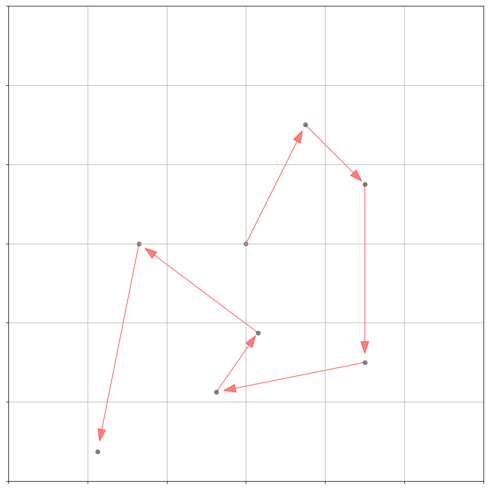
We can thus proclaim the following, somewhat un-mathematical property of this rambunctious little particle: \(\begin{align} \underbrace{dx_t}_{\text{change in space}} = \overbrace{\epsilon}^{\text{random move}} \underbrace{"dt"}_{\text{some change in time}} \end{align}\)
There are a couple of things to observe here:
- First we introduced a random variable $\epsilon$ which follows some probability distribution.
- Secondly, through the infinitesimal differentials on both sides we equated the random move in space with the duration of the movement just like in a differential equation.
- Thirdly, the infinitesimal movements of $x_t$ through time are completely independent since $\epsilon$ is sampled uncorrelated through time.
It turns out that if we choose the random movements $\epsilon$ and the change in time $”dt”$ smartly, we can derive convenient theoretical properties about the movement of the little random particle $x_t$.
Since $\epsilon$ is a random variable at any point in time, the position of $x_t$ will never be predictable with absolute certainty. Instead we have to treat the position of the particle $x_t$ itself as a random variable, the behavior of which is governed by the differential equation above.
First up is the choice of $\epsilon$. The usage of the Normal distribution $\mathcal{N}(\mu, \sigma)$ is prevalent in a lot of modelling approaches due to the convergence of sequences of random variables and it furthermore has nice theoretical properties. For that reason we will model the probability of the random movement $\epsilon$ with a standard normal distribution, namely $\epsilon \sim \mathcal{N}(0,1)$.
Secondly we will choose the “amount of time $dt$” to actually be $\sqrt{dt}$, the reason of which will be clear in an instant.
Thirdly, we want the particle to start at zero, so $x_0 = 0$.
Given these modelling assumptions, we are interested where the particle could turn up at a later point in time, so we want to know what $x_T$ is: \(\begin{align} x_T &= x_0 + \int_{t=0}^T dx_t \\ &= \underbrace{x_0}_{\text{$=0$}} + \int_{t=0}^T \epsilon \sqrt{dt} \\ &= \int_{t=0}^T \epsilon \sqrt{dt} \end{align}\)
But since $\epsilon$ is a random variable we actually have to treat the position of the particle at $x_T$ as a random variable. The most that we can do is thus to treat $x_T$ as a probability distribution for which we can compute the first two moments, the mean and the variance: \(\begin{align} \mathbb{E}\left[ x_T \right] &= \mathbb{E}\left[\int_{t=0}^T dx_t \right] \\ &= \int_{t=0}^T \underbrace{\mathbb{E}\left[ \epsilon \right]}_{\mathcal{N}(0,1)} \sqrt{dt} \\ &= 0 \end{align}\)
and \(\begin{align} \mathbb{V}\left[ x_T \right] &= \mathbb{V}\left[\int_{t=0}^T dx_t \right] \\ &= \int_{t=0}^T \underbrace{\mathbb{V}\left[ \epsilon \sqrt{dt} \right]}_{\mathbb{V}[a X] = a^2 \mathbb{V}[X]} \\ &= \int_{t=0}^T dt \underbrace{\mathbb{V}\left[ \epsilon \right]}_{\epsilon \sim \mathcal{N}(0,1)} \\ &= \int_{t=0}^T dt \\ &= T \end{align}\)
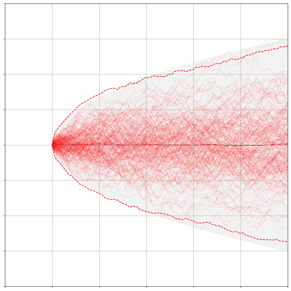
We can validate the properties of the Wiener process experimentally through what a good friend of mine calls “computational evidence”:
with the following code
T = 1000
dt = 1
MC = 200

mu = 0.0
sigma = 0.1

def drift(x, mu, dt):
	return mu*dt

def diffusion(x, sigma, dt):
	return sigma * dt**0.5*np.random.randn(*x.shape)

# start at zero
x = [np.zeros(MC)]

# simulate Brownian Motion in parallel
for _ in range(T):
	x.append(x[-1]+drift(x[-1], mu, dt) + diffusion(x[-1], sigma, dt))

x = np.array(x)

fig = plt.figure(1)
ax = fig.add_subplot(111)

# plot all the trajectories
_ = ax.plot(x, color='red', alpha=0.1)

# compute the analytical means and variances of the Brownian Motion
analytic_var = np.arange(0,T)*dt*sigma**2
analytic_std = analytic_var**0.5
analytic_mean = np.arange(0,T)*dt*mu

# compute the empirical mean and variance from the sampled Brownian Motion
empiric_var = x.var(axis=1)
empiric_std = empiric_var**0.5
empiric_mean = x.mean(axis=1)

ax.plot(empiric_mean + 3*empiric_std, ls='--', color='red')
ax.plot(empiric_mean - 3*empiric_std, ls='--', color='red')
ax.plot(x.mean(axis=1), ls='-.', color='red')

ax.fill_between(x=np.arange(0,T),y1=analytic_mean+3*analytic_std, y2=analytic_mean+-3*analytic_std, color='gray', alpha=0.1)
plt.plot(analytic_mean, color='gray', ls='-.')

ax.grid(True)
ax.set_xlim(-20,100)
ax.set_ylim(-4,4)
ax.set_xticklabels([],[])
ax.set_yticklabels([],[])
plt.show()
We can observe both the sampled mean and the variance (in red) of our 100 Wiener processes match the expected mean and variance (in gray) up to the noise that we introduce through sampling. Basically all the paths stay around zero where they start and they spread out according to our analytically computed variance of $\mathbb{V}[x_t] = t$ over time.
Since we chose $\epsilon$ and $”dt”$ smartly, we arrive at quite succinct definitions for the mean and variance of this random variable $x_T$. In fact, this specific kind of stochastic process has a specific name. By choosing the random movement $\epsilon \sim \mathcal{N}(0,1)$, the starting value $x_0=0$ and the time differential $\sqrt{dt}$ we have defined our little, rambunctious particle to follow a Wiener process which is a specific kind of stochastic process. The defining properties of a Wiener process $W_t$ ( $W_t$ being the common notation of a Wiener process) that describes the infinitesimal movement of a particle through $dx_t = \epsilon \sqrt{dt}$ are the following:
-
$W_0 = 0$
This means that the Wiener process always starts at zero. -
Independent increments: $\mathbb{C}[W_{t+u} - W_s, W_s] =0$ for $u \geq 0$ and $s \leq t$
Increments (the movement of the Wiener process) are independent from the past movements. $\mathbb{C}[\cdot , \cdot ]$ is the covariance between two random variables. -
Gaussian increments: $W_{t+u} - W_t \sim \mathcal{N}(0, u)$
The difference between any two realizations is Gaussian distributed accordingly to the time difference between these two realizations. -
Continuous paths in time $t$.
We can basically zoom infinitely far into the movements on the time axis and we will never find a discontinuous jump. Yet, due to it being a stochastic process it turns out that the Wiener process is not differentiable.
In order to be all set up for the final chapter of this post, we will define an infinitesimal version of the Gaussian increment property of the Wiener process: \(\begin{align} W_{t+u} - W_t \sim \mathcal{N}(0, u) \quad \Leftrightarrow \quad dW_t \sim \mathcal{N}(0,dt) \end{align}\)
Stochastic Differential Equations (= Differential Equations + Wiener Processes)
Once we understood differential equations and Wiener processes, we’ll realize that (basic) stochastic differential equations are just the combination of the two. We can thus define a stochastic differential equation as \(\begin{align} \underbrace{dX_t}_{\text{total change}} = \underbrace{\mu_t dt}_{\text{deterministic}} + \underbrace{\sigma_t dW_t}_{\text{stochastic}} \end{align}\)
which defines the infinitesimal change in the random variable $X_t$ at time $t$ as the combination of a deterministic change $\mu_t dt$ and a scaled Wiener process $\sigma_t dW_t \sim \mathcal{N}(0,\sigma_t^2 dt)$.
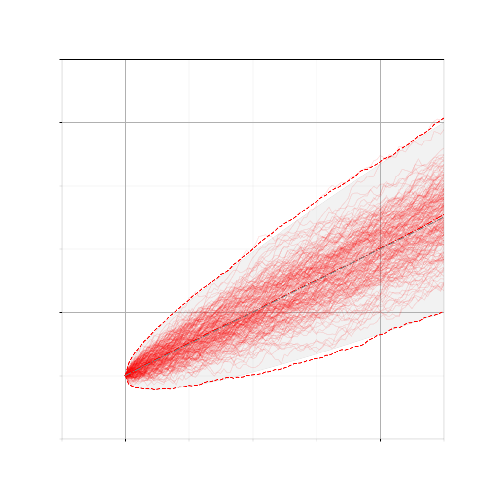
With a constant drift, this looks something like this:
through
T = 1000
dt = 1
MC = 200

mu = 0.1
sigma = 0.1

def drift(x, mu, dt):
	return mu*dt

def diffusion(x, sigma, dt):
	return sigma * dt**0.5*np.random.randn(*x.shape)

# start at zero
x = [np.zeros(MC)]

# simulate Brownian Motion in parallel
for _ in range(T):
	x.append(x[-1]+drift(x[-1], mu, dt) + diffusion(x[-1], sigma, dt))

x = np.array(x)

fig = plt.figure(1)
ax = fig.add_subplot(111)

# plot all the trajectories
_ = ax.plot(x, color='red', alpha=0.1)

# compute the analytical means and variances of the Brownian Motion
analytic_var = np.arange(0,T)*dt*sigma**2
analytic_std = analytic_var**0.5
analytic_mean = np.arange(0,T)*dt*mu

# compute the empirical mean and variance from the sampled Brownian Motion
empiric_var = x.var(axis=1)
empiric_std = empiric_var**0.5
empiric_mean = x.mean(axis=1)

ax.plot(empiric_mean + 3*empiric_std, ls='--', color='red')
ax.plot(empiric_mean - 3*empiric_std, ls='--', color='red')
ax.plot(x.mean(axis=1), ls='-.', color='red')

ax.fill_between(x=np.arange(0,T),y1=analytic_mean+3*analytic_std, y2=analytic_mean+-3*analytic_std, color='gray', alpha=0.1)
plt.plot(analytic_mean, color='gray', ls='-.')

ax.grid(True)
ax.set_xlim(-20,100)
ax.set_ylim(-4,4)
ax.set_xticklabels([],[])
ax.set_yticklabels([],[])
plt.show()
For such drift-diffusion processes, or more specifically Ito drift-diffusion processes, we can compute the analytical mean and variance of how $X_t$ will be distributed in the future. To keep things simple, we will work with a constant mean $\mu = \mu_t$ and diffusion $\sigma = \sigma_t$. Solving the SDE amounts to: \(\begin{align} X_T &= \int_{t=0}^T dX_t \\ &= \int_{t=0}^T \mu dt + \sigma dW_t \\ &= \mu \int_{t=0}^T dt + \sigma \int_{t=0}^T dW_t \\ &= \mu T + \sigma \int_{t=0}^T dW_t \\ &= \mu T + \sigma W_T \\ \end{align}\)
Similarly to earlier, the Brownian motion $W_T \sim \mathcal{N}(0,T)$ is a random variable, which entices us to compute the mean and variance of the term above: \(\begin{align} \mathbb{E}[X_T] &= \mathbb{E}[\mu T + \sigma W_T] \\ &= \mu T + \sigma \mathbb{E}[W_T] \\ &= \mu T \end{align}\) and \(\begin{align} \mathbb{V}[X_T] &= \mathbb{V}[\mu T + \sigma W_T] \\ &= \underbrace{\mathbb{V}[\mu T]}_{=0} + \mathbb{V}[\sigma W_T] \\ &= \sigma^2 \mathbb{V}[ W_T] \\ &= \sigma^2 T \\ \mathbb{Std}[X_T] &= \sigma \sqrt{T} \end{align}\)
which we were able to validate with our “computational evidence” in the plot above. The mean increases constantly as time progresses and the standard deviation above and below the mean increases asymptotically due to the $\sqrt{T}$.
This is a fairly simple SDE since we assume that $\mu_t$ and $\sigma_t$ are constant in time and do not depend on the value of $X_t$. Things get significantly more interesting when both $\mu_t$ and $\sigma_t$ change over time depending on the value of $X_t$ such that we are working with \(\begin{align} dX_t = \mu(t, X_t) dt + \sigma(t, X_t) dW_t \end{align}\)
The drift $\mu(t, X_t)$ and $\sigma(t, X_t)$ can now be potentially highly non-linear and complex functions which could even take in other stochastic processes as additional input. But Ito’s lemma, Ornstein-Uhlenbeck processes and Geometric Brownian Motion are topics for another time …
For the distributional view of the same dynamics — i.e. how the entire probability density $p(x,t)$ evolves in time rather than a single trajectory — see the Fokker-Planck equation and the Kramers-Moyal expansion. For the time-reversed counterpart used in generative diffusion models, see Simple Reverse-Time SDEs.