The Reparameterization Trick
Outsourcing Stochasticity and Making Normal Distributions Differentiable
Let’s assume we have normal standard distribution $\mathcal{E} \sim \mathcal{N}(0,1)$. We can draw lots of samples from it which will be distributed just like the parameterized distribution.
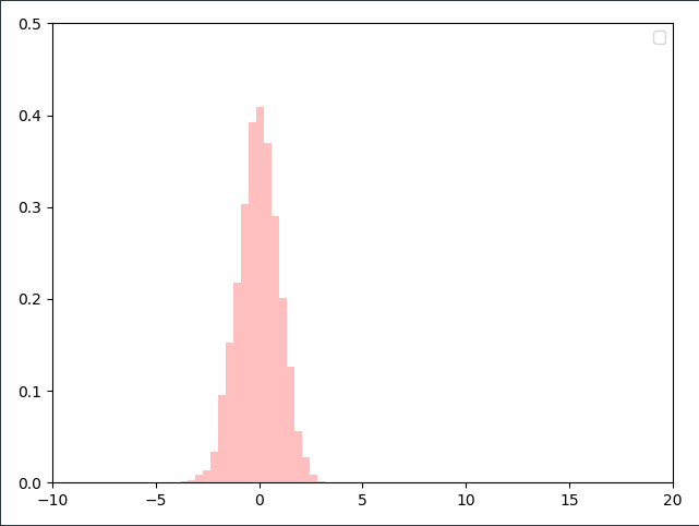
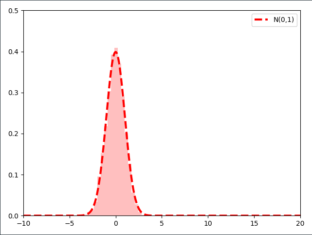
Unsurprisingly, the distribution of the samples follows the parameterized Normal distribution $\mathcal{N}(\mu=0, \sigma=1)$. If we were to sample millions of samples from the distribution and use a ever finer resolution of the histogram we would arrive at a perfect $\mathcal{N}(\mu=0, \sigma=1)$ distribution.
Let’s pick three samples $\epsilon_1, \epsilon_2, \epsilon_3$ from that standard normal distribution
\[\epsilon_1 = -0.5 \\ \epsilon_2=0.5 \\ \epsilon_3=1\]What would happen if we were to multiply these three samples with a constant number $\sigma=3$? Well since it is a linear transformation it should be a straight forward multiplication
\[\sigma \cdot \epsilon_1 = -1.5 \\ \sigma \cdot \epsilon_2 = 1.5 \\ \sigma \cdot \epsilon_3 = 3\]Let’s visualize this multiplication with a fixed number for thousands of samples $\epsilon$ from the standard normal distribution. In the next image I normalized the samples such that we’re working with a distribution:
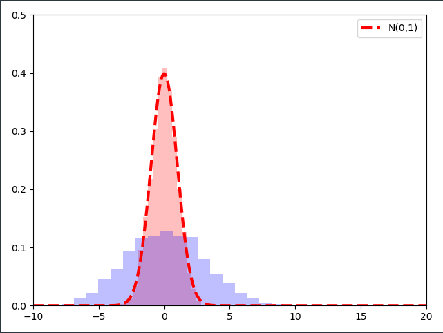
As it turns out, multiplying the samples of a $\mathcal{N}(0,1)$ distribution with a constant number $\sigma$ results in a Normal distribution with the standard deviation $\sigma$!
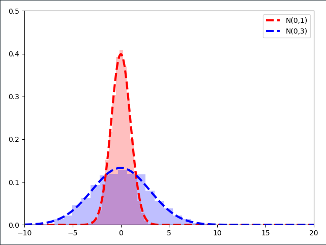
The second step of the reparameterization step is to ask ourselves what would happen if we added a constant number $\mu =10$ to the samples drawn from $\mathcal{N}(0,1)$ which are already multiplied with $\sigma$.
\[\mu + \sigma \cdot \epsilon_1 = 8.5 \\ \mu + \sigma \cdot \epsilon_2 = 11.5 \\ \mu + \sigma \cdot \epsilon_3 = 13\]Let’s visualize this linear transformation on all the samples we drew from $\mathcal{N}(0,1)$ and multiplied with $\sigma=3$.
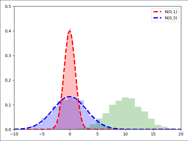
As it turns out, if we plot the Normal distribution $\mathcal{N}(10,3)$ on top of our scaled and shifted standard normal samples, we obtain the same distribution!
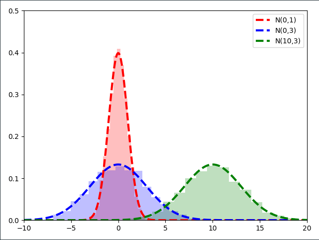
After some eye-candy we can tackle the above-mentioned transformation analytically. We transform any Standard-Normally distributed random variable $\mathcal{E} \sim \mathcal{N}(0,1)$ by scaling it first with $\sigma$ and shifting it afterwards with $\mu$ into a Normally distributed random variable $w \sim \mathcal{N}(\mu, \sigma)$ through the linear transformation
\[\begin{align*} w = t_1 (\mathcal{E}, \mu, \sigma) = \mu + \mathcal{E} \cdot \sigma \end{align*}\]Before we can dive into the gradients and properties we have to introduce one more non-trivial trick: keeping the standard deviation strictly positive. This can be achieved by reparameterizing the standard deviation itself with the transformation
\[\begin{align*} \sigma = t_2(\rho) = \log(1+\exp(\rho)) \quad ; \sigma \in \mathbb{R}^+, \rho \in \mathbb{R} \end{align*}\]The transformation is important as it allows $\sigma$ to be optimized freely without having to check after every optimization step, whether it is still positive. The parameter $\rho$ can be optimized freely from $-\infty$ to $+\infty$ and only the $\log-\exp$ transformation above turns it into a strictly positive number. For readability we will only use $\rho$ when it’s absolutely necessary since most people are fairly accustomed to the $\sigma$ notation of normal distributions.
The important analytical property of this reparameterization is that we can take gradients with respect to its parameters. Let’s create a simple example of linear regression of some input $x \in \mathbb{R}$ with a weight $w \sim \mathcal{N}(\mu,\sigma)$:
\[\begin{align*} \hat{y} = f(x) = w \cdot x = (\mu + \mathcal{E} \cdot \sigma) \ x \end{align*}\]Since $t_1$ is nothing else than a linear transformation we can easily take the gradients with respect to its parameters just as we would do with any other linear function. The objective function for the toy example which follows is
\[\begin{align*} \mathcal{L}(\hat{y}, y) &= \mathcal{L}( f(x, w), y ) \\\\ &= (w\cdot x - y)^2 \\\\ &= ((\mu + \mathcal{E} \cdot \sigma) \ x - y)^2 \end{align*}\]After the double reparameterization of $w$ with $t_1$ and $t_2$ we can compute the gradient for the deterministic parameters $\mu, \rho$ for the given cost function. This is possible because we ‘outsourced’ the stochasticity of the distribution $w \sim \mathcal{N}(\mu, \sigma)$ into the Standard Normal random variable $\mathcal{E}$. We are not interested in the stochasticity of $\mathcal{E} \sim \mathcal{N}(0,1)$ but in the parameters $\mu, \sigma$. All the transformations of the variational parameters above are encapsulated in the cost function below:
\[\begin{align*} \mathcal{L}(\hat{y}, y) &= \mathcal{L} (f(x, t_1(\mathcal{E}, \mu, t_2(\rho))), y) \end{align*}\]All we have to do is to apply the chain rule and work from outside towards the inside of the nested functions $\mathcal{L}, f, t_1$ and $t_2$. This is what is commonly called reverse-mode auto differentiation and is applied in neural networks in the backpropagation algorithm. The gradient for the variational parameter $\mu$ can be computed via:
\[\begin{align*} \frac{\partial \mathcal{L}}{\partial \mu} &= \frac{\partial \mathcal{L}}{\partial f} \frac{\partial f}{\partial w} \frac{\partial w}{\partial t_1} \frac{\partial t_1}{\partial \mu} \\\\ \frac{\partial \mathcal{L}(\hat{y}, y)}{\partial \mu} &= \frac{\partial \mathcal{L}(\hat{y}, y)}{\partial f(x, w)} \cdot \frac{\partial f(x, w)}{\partial w} \cdot \frac{\partial w}{\partial t_1(\mathcal{E}, \mu, \sigma)} \cdot \frac{\partial t_1(\mathcal{E}, \mu, \sigma)}{\partial \mu} \\\\ &= 2(\hat{y}-y) \cdot x \cdot 1 \cdot 1 \end{align*}\]and to obtain the gradient of the cost function with respect to $\rho$ we compute:
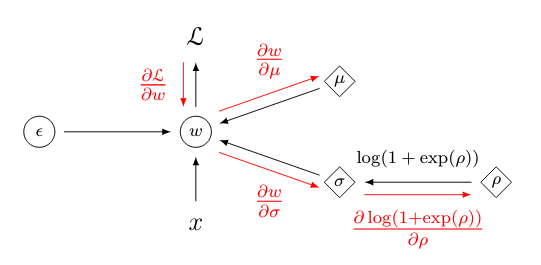
\[\begin{align*} \frac{\partial \mathcal{L}}{\partial \rho} &= \frac{\partial \mathcal{L}}{\partial f} \cdot \frac{\partial f}{\partial w} \cdot \frac{\partial w}{\partial g} \cdot \frac{\partial g}{\partial t_2} \cdot \frac{\partial t_2}{\partial \rho} \\\\ \frac{\partial \mathcal{L}(\hat{y}, y)}{\partial \rho} &= \frac{\partial \mathcal{L}(\hat{y}, y)}{\partial f(x, w)} \cdot \frac{\partial f(x, w)}{\partial w} \cdot \frac{\partial w}{\partial t_1(\mathcal{E}, \mu, \sigma)} \cdot \frac{\partial t_1(\mathcal{E}, \mu, \sigma)}{\partial t_2(\rho)} \cdot \frac{t_2(\rho)}{\partial \rho} \\\\ &= 2(\hat{y}-y) \cdot x \cdot 1 \cdot \mathcal{E} \cdot \frac{1}{1 + \exp(-\rho)} \end{align*}\]In essence, it is simply an extended chain rule where we not only have to backprop to the used weight $w$ but further through the reparameterization $t_1$ to obtain the gradient for $\mu$ and even further through the reparameterization $t_2$ to obtain the gradient for $\rho$. Below is a graphical representation of how the gradient is first backpropagated to the linear product $w \cdot x$ and then subsequently to the variational parameters $\mu, \rho$. Since we transform $\rho$ such that it will be in $\mathbb{R}^+$ with $t_2( \cdot )$ we also have to backpropagate through the transformation to obtain the gradient for $\rho$.

The final point is a little code snippet which can be analyzed without much plotting
import numpy as np

#Generate 10 data points between 0 and 5
x = np.linspace(0,5,10)
# Scale each data point with 3 such that we get a linear function with slope 3
y = 3*x

#Initialize the variational parameters mu and rho
mu = -3
rho = 1

#Set a learning rate
lr = 0.05

# Do a couple of epochs
for epoch in range(20):
    #Iterate over the training data
    for i, (label, data) in enumerate(zip(y, x)):

                #Sample from the standard normal distribution N(0,1)
                e = np.random.randn(1)
                #Transform the unconstrained variational parameter \rho into \sigma
                std = np.log(1+np.exp(rho))

                #Make a prediction with the sampled weight w=mu + e*std
                pred = (mu + e*std) * data

                #Backprop gradients onto the variational parameters
                mu = mu - lr * (pred - label) * data
                rho = rho - 3*lr * e/(1+np.exp(-rho)) * (pred - label) * data

                print('Episode {} | Data Point {}: μ: {:.2f}, σ: {:.02f}'.format(epoch, i, mu.squeeze(), std.squeeze()))
Running the little script we can see that the values were initialized with $\mu=-3$ and $\sigma=1.31$. After a couple of iterations the parameters converge on the correct values of $\mu=3$ and $\sigma=0$.
| Episode 0 | Data Point 0: μ: -3.00, σ: 1.31 |
| Episode 0 | Data Point 1: μ: -2.93, σ: 1.31 |
| Episode 0 | Data Point 2: μ: -2.77, σ: 1.42 |
| Episode 0 | Data Point 3: μ: -1.75, σ: 2.11 |
| Episode 0 | Data Point 4: μ: -0.66, σ: 0.69 |
| Episode 0 | Data Point 5: μ: 0.64, σ: 1.15 |
| Episode 0 | Data Point 6: μ: 1.62, σ: 1.67 |
| Episode 0 | Data Point 7: μ: 3.62, σ: 2.40 |
| Episode 0 | Data Point 8: μ: 3.80, σ: 0.44 |
| Episode 0 | Data Point 9: μ: 2.20, σ: 0.33 |
| Episode 1 | Data Point 0: μ: 2.20, σ: 0.05 |
| Episode 1 | Data Point 1: μ: 2.21, σ: 0.05 |
| Episode 1 | Data Point 2: μ: 2.26, σ: 0.05 |
| Episode 1 | Data Point 3: μ: 2.36, σ: 0.05 |
| Episode 1 | Data Point 4: μ: 2.52, σ: 0.05 |
| Episode 1 | Data Point 5: μ: 2.69, σ: 0.05 |
| Episode 1 | Data Point 6: μ: 2.90, σ: 0.05 |
| Episode 1 | Data Point 7: μ: 2.95, σ: 0.05 |
| Episode 1 | Data Point 8: μ: 3.02, σ: 0.05 |
| Episode 1 | Data Point 9: μ: 2.92, σ: 0.05 |
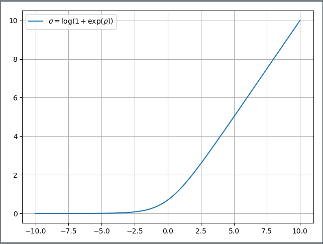
It should be noted that the through the $\sigma = \log(1+\exp(\rho))$ transformation the gradient with respect to $\rho$ becomes very, very small for large negative values of $\rho$. The transformation $t_2$ is referred to as the ‘Softplus’ activation function is shown below. We can see that while $\rho$ is freely optimizable the ‘Softplus’ function flattens out for negative values of $\rho$ and the resulting gradient is almost zero. So we’re basically at the same spot deep learning was at 10 years ago with the vanishing gradient problem in very deep neural networks. The Glorot-Activation and ReLU activation functions solved it and maybe somebody will develop a new fancy reparameterization for the variational parameter $\rho$. =) That’s why it will never really converge to absolute 0, but that’s a trade-off we’re willing to make if we’re able to scale variational inference to large data sets.
