Bernoulli to Poisson Point Processes

Recently I got interested in Poisson point processes which model the probabilities of phenomena or objects in some type of space. These types of spaces can be anything from a real line to a Cartesian plane.

The most direct application of point processes is queueing theory with which we can model how many packages will arrive at a certain node in a network over time. Mathematically it looks like this: \(\begin{align} \mathbb{P}\left[ N(t) = k \right] = \frac{( \ \lambda t \ )^k}{k!} e^{-\lambda t} \end{align}\) where $t$ is the time, $N(t)$ is a counting process and $\lambda$ is the intensity of the Poisson point process. The first time I saw this probability, I frankly didn’t know what I was supposed to make of this probability so I started reading. And the following paragraphs are the trip I took to understand the probability above.

Counting Process

Let us first start with the notion of discrete jumps in stochastic processes.

A counting process is a stochastic process \(\{ N(t), t \in \mathbb{R}_+ \}\) with values that are non-negative, integer and non-decreasing.

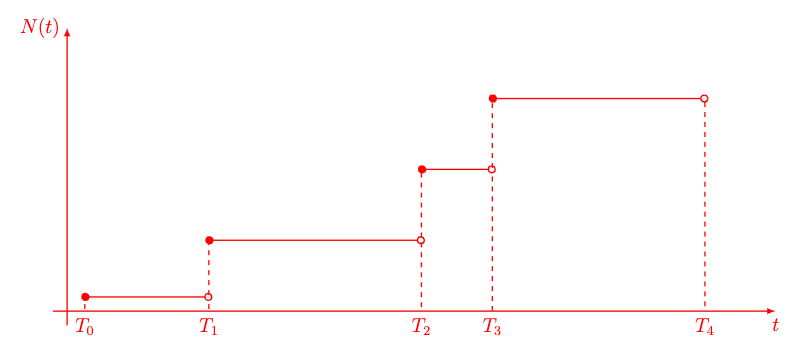
The gist of the figure above is that a counting process increases monotonically over time $t \in \mathbb{R}_+$ with integer steps of 1. Mathematically, a counting process $N(t)$ is defined in the following way \(\begin{align} N(t) &= \sum_{k \geq 1} \mathbb{1}_{(T_k, \infty)} (t) \\ \mathbb{1}_{(T_k, \infty)} (t) & = \begin{cases} 1, & \text{if } \ t \geq T_k \\ 0, & \text{if } \ 0 \leq t \leq T_k \\ \end{cases} \end{align}\)

In order to determine $N(t)$ for some specific value of $t$, all you have to do is to compare $t$ to each $T_k$ that you have recorded, and if $t\geq T_k$, add it to $N(t)$. The stochastic part comes from the fact that the jump times $T_k$ are stochastic and follow some distribution.

Bernoulli Distribution

A binary random variable \(X \in \{0,1\}\) follows a Bernoulli distribution if it takes on the value $1$ with probability $p$ and the value $0$ with probability $q=1-p$. More succinctly, we can write \(\begin{align} \mathbb{P}\left[X=0 \right] &= 1-p = q \\ \mathbb{P}\left[X=1 \right] &= p \\ \mathbb{P}\left[X=k \right] &= p^k (1-p)^{1-k} \quad \text{with} \quad k \in \{0,1\} \end{align}\)

For a single binary experiment, the Bernoulli distribution models the probability that each outcome has. But what if we would like to conduct multiple experiments? Enter the Binomial distribution.

Binomial Distribution

Let’s say you want to conduct $n$ experiments with a binary outcome (yes/no, true/false, 1/0 etc) given some probability of success $p$ and some probability of defeat $q=1-p$. Obviously, you can run the $n$ separate experiments and count the number of total successes from your $n$ experiments. The expected number of successes for $n$ trials with a success probability $p$ amounts to $np$. For example, if $n=100$ and $p=0.6$, on average we will obtain $k=60$ successful trials.

But a more interesting question looms in the background. It is certainly nice to know that if we run those $n=100$ trials a million times, we will eventually converge to $k=60$ succesfull runs per $n=100$ trials with a success probability of $p=0.6$. But we shouldn’t forget that each time we run the $n=100$ experiments, we will obtain a different result for \(k \in \{0, n\}\). So it could certainly happen that one run has exactly $k=60$ while the other run has $k=43$.

In the grander scope of things, we would like to know what the probabilities are for each success rate $k$. More specifically, we are interested in the probability of $\mathbb{P}\left[k=60 \right]$ trials versus $\mathbb{P}\left[k=43 \right]$, for example.

This appears to be similar to the Bernoulli distribution except that we do $n$ trials instead of just one trial, \(\begin{align} \mathbb{P}\left[k,n, p \right] &\propto p^k (1-p)^{n-k} \quad \text{with} \quad k \in \{0,n\}. \end{align}\)

The proportional sign was chosen on purpose to denote that this does not denote a valid distribution. We made no assumption with regards to the ordering of the successful trials. All we are interested in is the total number of successful trials and not the order. Naturally, one could simply assume an ordering in which all successful trials occur subsequently and the final $n-k$ trials are the unsuccessful trials. But since the trials are inherently stochastic, it could also occur that the first $n-k$ trials are unsuccessful and only the last $k$ trials are successful or any possible other ordering with $k$ successful trials and $n-k$ unsuccessful trials. Since we are not interested in the ordering, we have to basically sum up all the possibilities of ordering.

We can derive the number of possible orderings by thinking of how the successful trials $k$ are drawn from the number of trials $n$. First of all we know that for $k$ successful draws, any combination of exactly $k$ successful draws is permissible. So we could have \((47, 1, 13, \ldots, 16 )\) or \((1, 2, 3, \ldots, 98 )\) as long as number of draws in those tuples is exactly $k$. The first time we draw, we have 100 options, but the second time we draw we only have 99 options left and the the third time we draw we only have 98 left and so on. In order to express this mathematically, we can conclude the following with regards to “k out of n” orderings: \(\begin{align} \text{"60 out of 100"} &= 100 \cdot 99 \cdot 98 \cdot \ldots \cdot 42 \cdot 41\\ &= \frac{100 \cdot 99 \cdot 98 \cdot \ldots \cdot 2 \cdot 1 }{40 \cdot 49 \cdot \ldots \cdot 2 \cdot 1} \\ &= \frac{100!}{(100-60)!} \end{align}\)

So in general we can conclude that if we want to draw $k$ ordered, successful trials out of $n$ total trials we have \(\begin{align} \text{"k out of n"} &= \frac{n!}{(n-k)!}. \end{align}\)

But there is a catch. So far we have only considered cases of unique orderings, such as \((47, 1, 13, 16)\) and \((1, 47, 13, 16 )\) which have the same elements just in a different order. But we are only interested whether the trials are successful, not how the successful trials are ordered. The notion of interest is whether the draws occur in the set such as \(\{(47, 1, 13, 16), (1, 47, 13, 16 ) \} \subset \{1, 13, 16, 47 \}\) (which I ordered for convenience’s sake) and not their order. Fortunately, there is a quick fix to this: Simply divide by the number of possible permutations of the set $k!$: \(\begin{align} \binom{n}{k} = \underbrace{\frac{1}{k!}}_{\text{unordered correction}} \underbrace{\frac{n!}{(n-k)!}}_{\text{# of unique orderings}} \end{align}\)

The binomial coefficient is the normalization constant which corrects the original probability $p^k (1-p)^{n-k}$ by the number of possible permutations.

Thus we obtain the binomial distribution which states \(\begin{align} \mathbb{P}\left[k,n, p \right] &= \binom{n}{k} p^k (1-p)^{n-k} \\ &= \frac{n!}{k! (n-k)!} p^k (1-p)^{n-k} \end{align}\) which tells us what the probability of a certain number of successful trials $k$ is, if we run $n$ trials with a success rate of $p$.

Poisson Distribution

The binomial distribution defines the probability of $k$ successful trials for a fixed set of trials $n$ for a success probability $p$. For example, we can observe a logistics network and can ask every second whether a package has arrived or not. Remember that the binomial distribution is only defined for binary outcomes. We can then model how many packages arrive per minute or even hour by multiplying the number of seconds per minute or hour by the probability $p$ of a package arriving.

That time partition is still discrete, though, and the real world is continuous. We can let $\lim n \rightarrow \infty$ to model an infinitely fine partition of time. But now we’re confronted with the inconvenient \(\lim_{n \rightarrow \infty} np = \infty\) which we can’t really work with. instead we can redefine the probability \(p = \frac{\lambda}{n}\) with an intensity $\lambda$ which will be invariant to time, so to speak, because \(\lim_{n \rightarrow \infty} np = \lim_{n \rightarrow \infty} n \frac{\lambda}{n} = \lambda\).

We can then substitute $p = \frac{\lambda}{n}$ into the binomial distribution and see where that takes us: \(\begin{align} \lim_{n \rightarrow \infty} \mathbb{P} \left[ n, k, p \right] &= \lim_{n \rightarrow \infty} \frac{n!}{k!(n-k)!} p^k (1-p)^{n-k} \\ &= \lim_{n \rightarrow \infty} \frac{n!}{k!(n-k)!} \left( \frac{\lambda}{n} \right)^k \left( 1-\frac{\lambda}{n} \right)^{n-k} \\ &= \lim_{n \rightarrow \infty} \frac{n!}{k!(n-k)!} \left( \frac{\lambda}{n} \right)^k \left(1-\frac{\lambda}{n} \right)^{n-k} \\ &= \frac{\lambda^k}{k!} \lim_{n \rightarrow \infty} \frac{n!}{k!(n-k)!} \frac{1}{n^k} \left(1-\frac{\lambda}{n} \right)^{n-k} \\ &= \frac{\lambda^k}{k!} \lim_{n \rightarrow \infty} \frac{n!}{(n-k)!} \frac{1}{n^k} \left(1-\frac{\lambda}{n} \right)^n \left(1-\frac{\lambda}{n} \right)^{-k} \\ &= \frac{\lambda^k}{k!} \lim_{n \rightarrow \infty} \frac{n \cdot (n-1) \cdot (n-1) \cdot \ldots \cdot (n-k)}{n^k} \left(1-\frac{\lambda}{n} \right)^n \left(1-\frac{\lambda}{n} \right)^{-k} \\ &= \frac{\lambda^k}{k!} \lim_{n \rightarrow \infty} \underbrace{\frac{n}{n} \cdot \frac{(n-1)}{n} \cdot \frac{(n-1)}{n} \cdot \ldots \cdot \frac{(n-k)}{n}}_{1 \text{ for } \lim_{n \rightarrow \infty}} \underbrace{\left(1+\frac{1}{\frac{n}{-\lambda}} \right)^{-\lambda \frac{n}{-\lambda}}}_{=e^{-\lambda}} \underbrace{\left(1+\frac{\lambda}{n} \right)^{-k}}_{1 \text{ for } \lim_{n \rightarrow \infty}} \\ &= \frac{\lambda^k}{k!} e^{-\lambda} \\ &= \text{Poisson} [ \lambda] \end{align}\)

The Poisson distribution is a discrete distribution with support $k \in \mathbb{N}_+$ that quantifies the probability of $k$ events happening in an interval of time or space with $\lambda$ denoting the intensity of events (like how often they occur).

Poisson Point Process

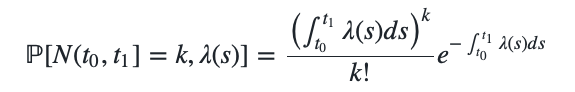
The Poisson distribution above allows us to compute the probability of $k$ events for a given fixed interval of time or space. We can generalize the Poisson distribution to a Poisson point process over varying intervals by integrating over the (possibly changing) intensities that the space exhibits. For a Poisson point process defined over a time interval $(t_0, t_1]$, we could compute the number of expected events by integrating the intensity of $\lambda(t)$ which is a function of time $t$: \(\begin{align} \mathbb{P}[N(t_0, t_1]=k, \lambda(s)] = \frac{\left( \int_{t_0}^{t_1} \lambda(s) ds \right)^k}{k!} e^{-\int_{t_0}^{t_1} \lambda(s) ds} \end{align}\)

We can recover the original Poisson distribution through a homogeneous Poisson point process which has a constant $\lambda$ and for which the, in our case time, integral evaluates to $\int_{t_0}^{t_1} ds = 1$. In fact, a meaningful intensity $\lambda$ for a Poisson distribution can only be determined for a-priori defined, fixed interval of time or space. The Poisson point process is then the natural extension to varying intervals of time or space by defining a varying intensity $\lambda(s)$. A homogeneous Poisson point process for a fixed interval $\int_{t_0}^{t_1} = 1$ can be obtained through \(\begin{align} \mathbb{P}[N(t_0, t_1]=k, \lambda] &= \frac{\left( \int_{t_0}^{t_1} \lambda ds \right)^k}{k!} e^{-\int_{t_0}^{t_1} \lambda ds} \\ &= \frac{\left( \lambda \int_{t_0}^{t_1} ds \right)^k}{k!} e^{-\lambda \int_{t_0}^{t_1} ds} \\ &= \frac{\left( \lambda \right)^k}{k!} e^{-\lambda} \end{align}\)

The definition above unfortunately only tells us the number of events occuring over the entire interval $(t_0, t_1]$. What if we wanted to now the probability of an event happening at a singular moment $t$? We should remember that a Poisson point process can be interpreted as a counting process $N(t)$ since it starts at zero, is monotonically increasing and the probability of an event happening is randomly distributed with $\int_{t_0}^{t_1} \lambda(s) ds$ which simplifies to just $\lambda t$ for a constant intensity and $t_0 = 0$, $t_1 = t$. Our derivation showed us that if we expand the Bernoulli distribution to a Binomial distribution with an infinite number of trials we arrive at the Poisson distribution which lies at the heart of a Poisson point process. Nevertheless the counting process always increases by a single integer step. Thus we can ask the question what the probability is of an event at an arbitrary point in the interval.

We can therefore inquire about the probability of an event not happening, ergo $N(t_0, t_1]=0$: \(\begin{align} \mathbb{P}[N(t_0, t_1]=0, \lambda(s)] &= \frac{\left( \int_{t_0}^{t_1} \lambda(s) ds \right)^0}{0!} e^{-\int_{t_0}^{t_1} \lambda(s) ds} \\ &= e^{-\int_{t_0}^{t_1} \lambda(s) ds} \end{align}\) which is the probability that no event will occur until $t_1$. As the intensity is a strictly positive quantity, the integral $\int_{t_0}^{t_1} \lambda(s) ds$ increases monotonically over time until an event occurs. Naturally since the integral is monotonically increasing, the probability of no event is monotonically decreasing through the negated exponential. This is quite intuitive as it states that the probability of no event happening decreases monotonically as time progresses. On the flip side, this means that the probability of an event occuring is monotonically increasing as time progresses: \(\begin{align} \mathbb{P}[N(t_0, t_1]=1, \lambda(s)] &= 1 - e^{-\int_{t_0}^{t_1} \lambda(s) ds}. \end{align}\)

The reason why we analyze only a single event $k=1$ lies with the fact that the events are i.i.d. distributed which in case for the Poisson distribution means that the integral is reset after each event. This is the reason why we only integrate to $t_1$. Since $\mathbb{P}[N(t_0, t_1]=1, \lambda(s)]$ is a cumulative probability distribution as it approaches 1 in infinity, we call simply derive it with respect to $t_1$ to obtain the probability density function: \(\begin{align} \mathbb{P}[N(t_1)=1, \lambda(s)] &= \frac{d}{dt_1} \left[ 1 - e^{-\int_{t_0}^{t_1} \lambda(s) ds} \right] \\ &= \lambda(t_1) e^{-\int_{t_0}^{t_1} \lambda(s) ds}. \end{align}\)

Another fun fact of the Poisson process is that its derivative is in fact a Bernoulli distribution. To see this we inspect the Poisson process for an extremely small time frame $\lim_{\Delta t \rightarrow 0} [t, t+ \Delta t]$: \(\begin{align} \lim_{\Delta t \rightarrow 0} \mathbb{P}[N(t, t + \Delta t]=k, \lambda(s)] = \lim_{\Delta t \rightarrow 0} \frac{\left( \int_{t}^{t + \Delta t} \lambda(s) ds \right)^k}{k!} e^{-\int_{t}^{t + \Delta t} \lambda(s) ds} \end{align}\)

which for \(k=\{0, 1\}\) and a first order exponential series expansion \(e^x = \sum_{k=0}^\infty \frac{x^k}{k!}\) yields \(\begin{align} \lim_{\Delta t \rightarrow 0} \mathbb{P}[N(t, t + \Delta t]=0, \lambda(s)] &= \lim_{\Delta t \rightarrow 0} \frac{\left( \int_{t}^{t + \Delta t} \lambda(s) ds \right)^0}{0!} e^{-\int_{t}^{t + \Delta t} \lambda(s) ds} \\ & \approx e^{- \lambda(t)\Delta t} \\ & \approx 1 - \lambda(t) \Delta t \\ \lim_{\Delta t \rightarrow 0} \mathbb{P}[N(t, t + \Delta t]=1, \lambda(s)] & = \lim_{\Delta t \rightarrow 0} \frac{\left( \int_{t}^{t + \Delta t} \lambda(s) ds \right)^k}{k!} e^{-\int_{t}^{t + \Delta t} \lambda(s) ds} \\ & \approx \lambda(t) \Delta t e^{- \lambda(t)\Delta t} \\ & \approx \lambda \Delta t - \underbrace{\lambda(t)^2 \Delta t^2}_{=0, \Delta t \rightarrow 0} \\ &= \lambda \Delta t \end{align}\)

which are precisely the probabilities for a Bernoulli distribution.