Monte Carlo (git) Tree Search

There has been a tremendous interest in doing autoresearch with LLM agents. The core idea is that since LLM’s have intelligence (the amount for real world problem solving is still being debated), have infinite stamina and have access to the abundance of information on the web including all recent research, then they could automate parts of the research pipeline that we all do. Evidently, the writing was on the wall and there is a whole swath of start ups that try to capitalize on this idea with the idea of an AI scientist (Periodic Labs, FutureHouse etc).

LLM’s rely on the iterative filling of their context (to have context at all) and you can add a RAG system, but then you’re still dependent on what’s in your context. So whatever a LLM does to solve a problem is highly influenced by what’s in it’s context. Of course there is a lot of baseline intelligence in LLM’s, but the context is still a huge factor in what it can do.

But research is not a linear process in the same way that we linearly and monotonically fill up a context. Research consist of many rabbit holes, dead ends and resets. This resetting is something that LLM’s are not ideally placed to do due to the their dependence on the context when trying to find solutions to problems by trial and error.

That begs the question: can we wrap a harness around a LLM to make it more like a human researcher that’s able to deal with setbacks, rabbit hole failures and resetting the context when needed?

Graduate student descent

There’s an old joke in machine learning that the real optimization algorithm behind most papers isn’t Adam or SGD. It’s graduate student descent: a PhD student sits in front of a screen, semi-informed, and tweaks things. Bump the learning rate. Swap out a loss term. Try a slightly different architecture. Rerun. Squint at the validation number. Try again.

Most of this is busywork — hyperparameter fiddling, “what if I change this one thing,” waiting for the run to finish. Only a handful of the tries actually matter, and the student usually can’t tell in advance which ones, which is exactly why they have to keep trying.

Having done a PhD in machine learing I’m all too familiar with this process. I have spent countless hours doing this exact loop, it’s unfortunately necessary to get a good result, but it’s also mind numbing and not very fun when you haven’t found the magic combination yet. I doubt we’ll be able to do away with graduate student descent as machine learning is intrinsically a latent model problem where try to explain/model/predict data and generalize from it. If you’ve done machine learning research you’ll know th Bermuda triangle of hope between model architecture, parameter optimization and data quirks.

Your graduate student of choice would

• proposes a change, based on a hunch about what might help,
• evaluates it by running a training job and reading off a number,
• and then decides what to try next — usually by leaning into whatever’s been working, but every so often taking a flyer on a direction they’ve barely touched.

It’s a semi-informed search over the tree of possible experiments, steered by intuition and metrics. Intuition is hard to come by if you haven’t done a lot of research before, but LLM agents offer boundless stamina and will never stop trying stuff out. This has been epitomized in the Ralph loop where a semi-intelligent actor just hammers the problem over and over again. Or it’s your new grad student is still optimistic about the next experiment.

Branching and Resetting

The other modus operandi we usually face in research is that we often have to reset our context and start over. That’s the humiliating act of realizing that your ideas have failed and we need to figuratively and literally clean the white board.

Here’s my biggest gripe with using LLM’s for autoresearch: They’re hard at resetting their context and starting over in a principled way. The original idea of autoresearch by Karpathy was to use git to reset to the previous state if something failed but it still left the context unchanged. So fundamentally, while the code was reset the context wasn’t. It essentially set the autoresearch agent on a linear trajectory of git states with no way of completely changing track and pursuing a different line of research.

But git allows branching such that we could try different ideas from the same root node. We can try experiments and log the code state in the git tree and then branch off to try a different idea. Importantly, this allows us to keep a ledge or diary of sorts of the many experiments which can develop in a multitude of different ways. If we want to revisit a prior experiment, we simply have to checkout the git commit and we have the exact code state that was used to run that experiment. That allows us to jump around in the tree and pursue different lines of research.

Monte Carlo Tree Search

So up to now we’ve concluded that LLM are useful testing out ideas with unwavering enthusiasm and that git is a perfect way to log the experiments and keep track of the many different lines of research. The last missing piece of the puzzle is to combine the two in a principled way such that we can explore the tree of experiments in a way that balances exploration and exploitation.

A long while ago in 2017, I gave a talk on AlphaGo and the Monte Carlo Tree Search algorithm that they used as a fast rollout policy to explore the state space tree of a game of Go. Mind you, Go is a game with a huge state space and the number of possible moves is astronomical. So they used a combination of a neural network to evaluate the board state and a Monte Carlo Tree Search to explore the tree of possible moves.

In the Monte Carlo Tree Search algorithm we work fundamentally on a tree structure where each node is a state and each edge is a possible action that can be taken from that state.

MCTS is a way to explore the tree of possible states in a principled way that balances exploration and exploitation. In the case of AlphaGo we simply counted the number of times a node was visited and the number of wins that were achieved from that node.

As the saying goes “An image is worth a thousand words” so let’s look at the MCTS algorithm in a visual way:

← Prev

1 / 6Game tree

Next →

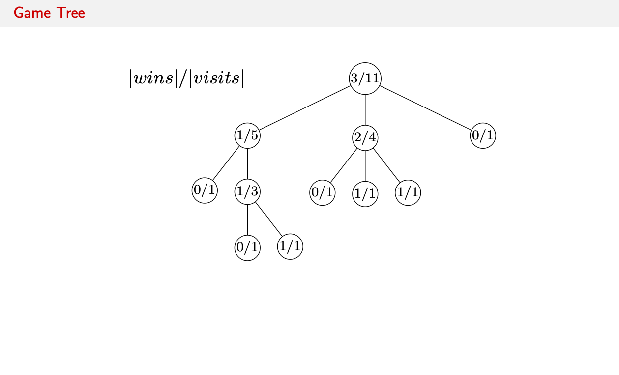
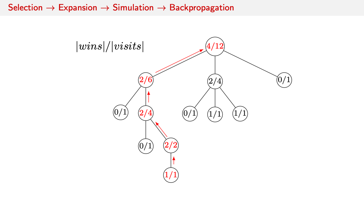
Initially we start out with a state tree with all the moves with their wins and visits.

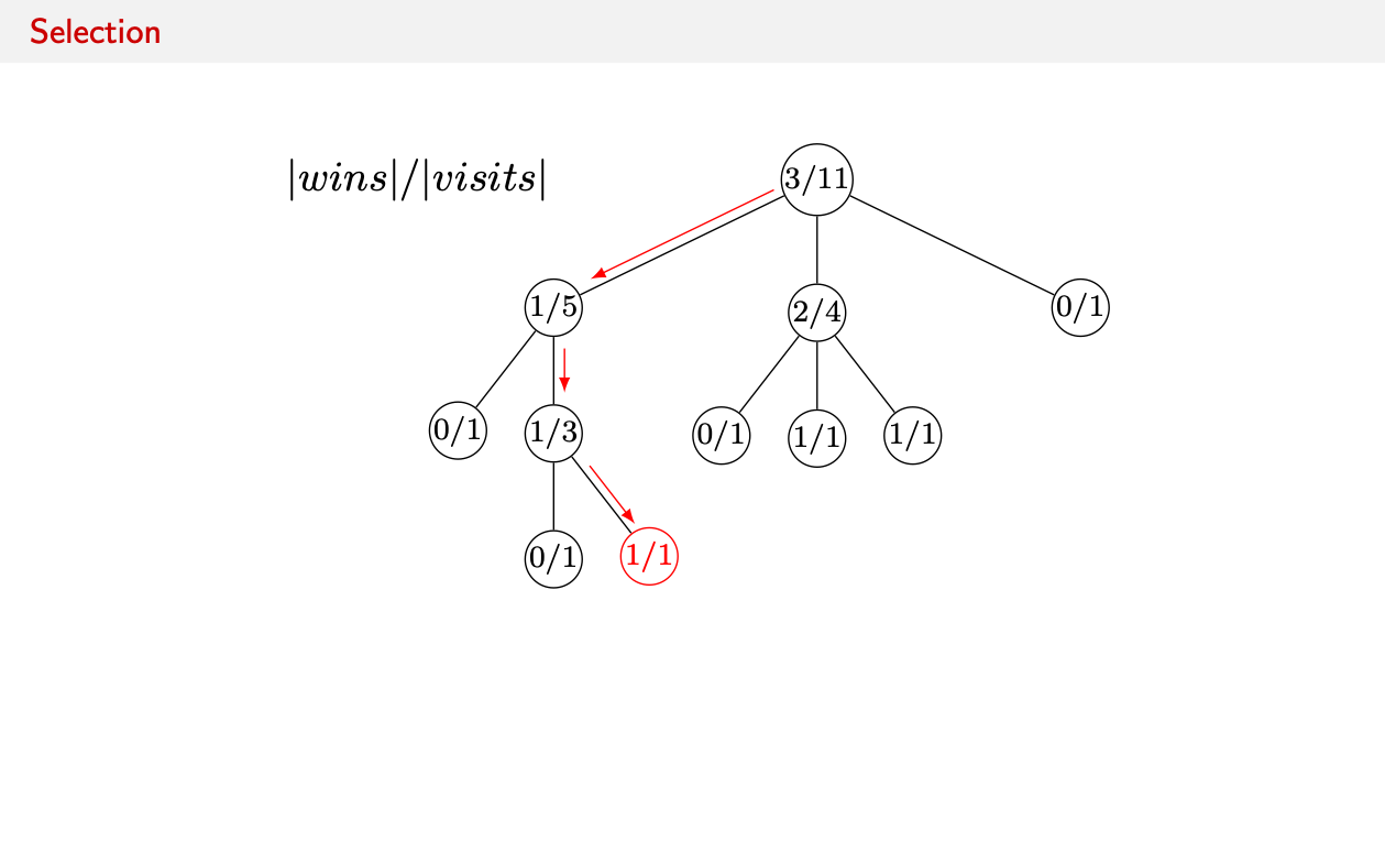
• Select: We use a formula to compare all non-terminal child nodes in the tree and decide to which child node to go first. In this simple case we simply compare the number of wins in the subtree to all visits of the subtree.
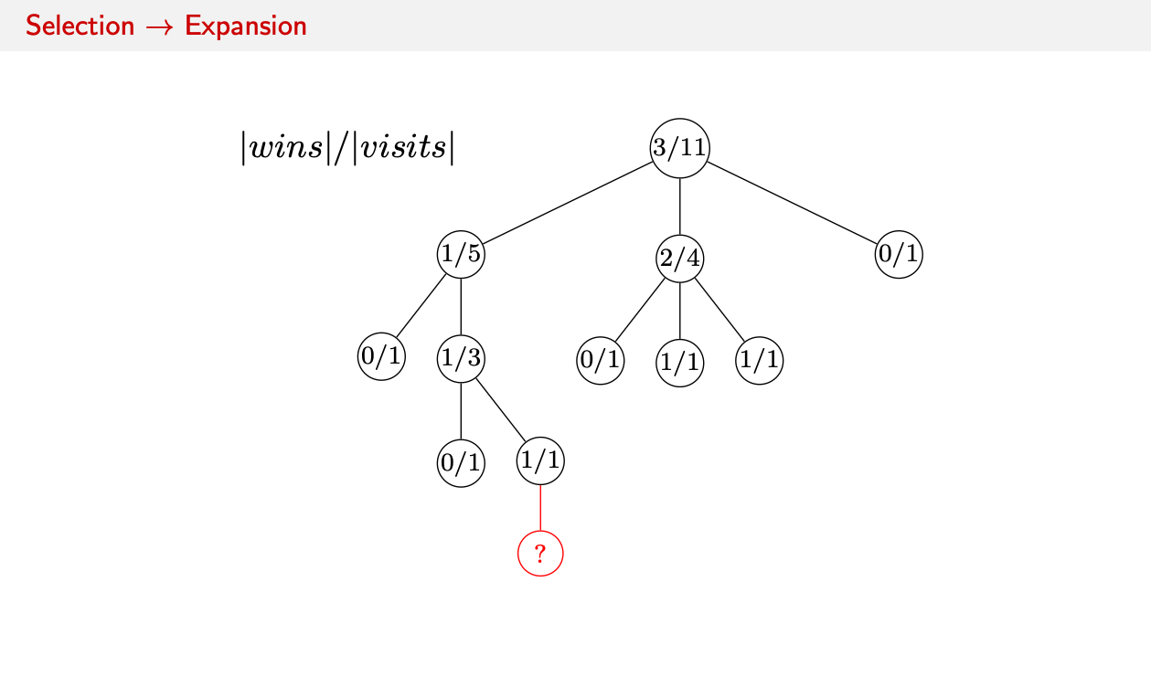
• Expand: Reaching a terminal leaf node, we chose an action on how to change the state. In Go we would place a stone on the game board.
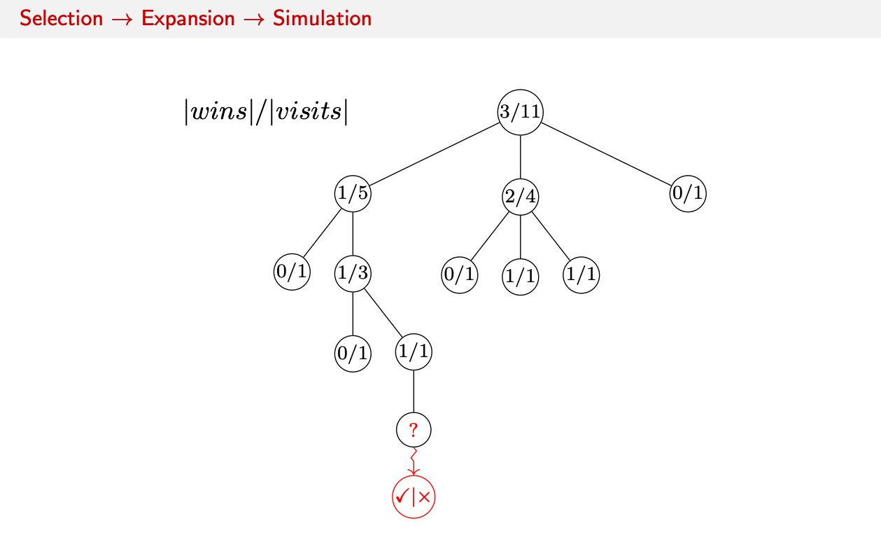
• Simulate: We then simulate the game from the new state to see the outcome. This could be a cheap and fast rollout policy until we win or loose.
• Backpropagate: We log the win (or loss) and backpropagate the ratio up the tree, automatically increasing the number of wins of any node between the leaf node and the root. This increases the percentage of wins all of those recursive subtrees.
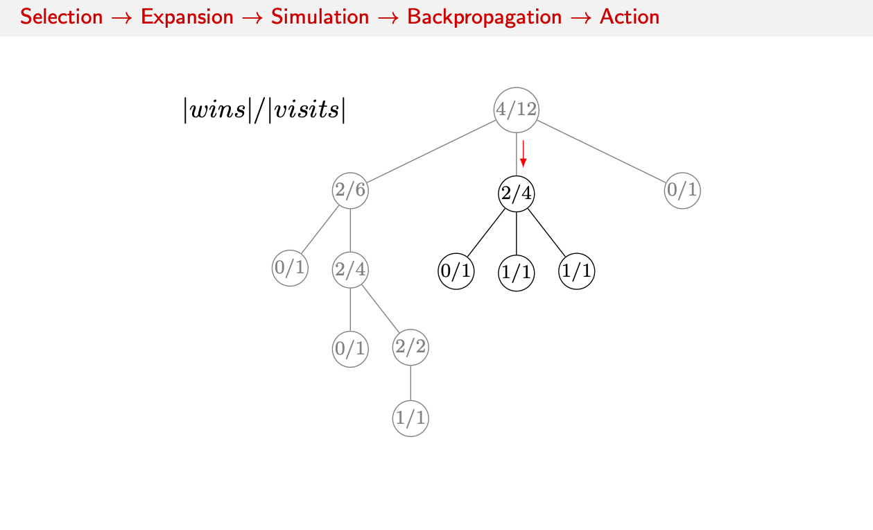
• Action: With one win or loss recorded, we can choose the best action based on the updated statistics. We use a policy that does a bit of exploration and chooses the middle subtree.

Below is an animation of a MCTS search for a simple analytical case to visualize the search character. The reward is a simple function of a binary action whether to add a 0 or a 1 to a string of length 5. The reward is the number of 1’s in the string. The search starts at the root node and explores the tree of possible strings until it finds the optimal string of all 1’s. After having found the gren and dark green combinations the algorithms keeps on exploring the lesser valuable paths to make sure that it doesn’t miss a better solution.

Translating MCTS to Autoresearch

MCTS gives us a principled way to explore a tree of possible states all originating from a common root node and searching the tree for the best state.

In order to get the performance of a particular node, we define a validation script that isn’t allowed to change and returns a single metric that gauges the performance of the state. This metric is then used to compare the performance of different nodes in the tree.

MCTS was originally formulated for games which have a binary outcome: win or loss. In machine learning research we often have a continuous outcome (loss) and we want to minimize that loss. The simple switch is to set an upper and lower (preferabbly zero but negative loglikelihoods can go lower) bound and then just rescaling the validated performance in those bounds to a [0,1] range.

The selection is a formula that compares the performance of all child nodes and chooses the best one to explore further. A particular node can have children which are already validated or (pre-generated) proposals which still require an expansion.

An expansion is the code change that we did that changes the code base of a particular node in the tree. This could be a change in the model architecture, a change in the loss function, a change in the optimizer or a change in the data set.

After each expansion we run the validation script to see how good our change performed. This is the simulation step in MCTS. Of course our proposal can be so bad that we run immediatley into NaN’s or other problems. In that case we simply ignore the proposal and mark it as failed. Failed nodes have no repercussion and are simply skipped in the selection step and represent a dead end.

Once the simulation/validation ran, we backpropagate the [0,1] value up the path between the leaf node and the root node, updating the performance of all nodes in between.

Here’s an interactive example with random best values. You can play it a couple of times ot see how

Notice how the search keeps coming back to the best branch — but never only that branch. Every so often it wanders off to try something it has mostly ignored. That tension, between milking what already works and checking on what you’ve neglected, is the whole game. Hold onto it; in a moment we’ll see the exact formula that produces it.

Keeping things simple

The idea is all nice but the devil’s in the detail as we all know.

For the implementation I opted for a some very hard boundaries.

• Simple: The whole setup should consist of a single functional file and maybe an additional utils file
• A Single Contract: There is no try/except (looking at you coding agents), defaults, if/else and catch mechanism. There is a single way to run this simple set up, if you don't it will fail.
• YAGNI (Recycling git): Git provides everything we need via inheritance, branching, checking out commits in a super convenient package. We will use as much of git as possible.
• Extendable Base Case: With the three paradigms above in a single functional python script, it can easily be extended for more complex scenarios to your liking.

Wait, how do we inject “intelligence” into the whole setup? It’s simple: we use the Python SDK for Copilot/Claude. With everything we’ve talked about so far, every step of the way is a simple prompt to the LLM with a very specific task and a very specific context. Essentially, we have a very clear idea of what we want to do and we can prompt the LLM to do it for us. The thing is that we can actually isolate the LLM to whatever it’s supposed to do and not let it wander off into the weeds of the code base. Since everything runs on git, we can run git commands manually from within the research loop, and start a coding session with the LLM to implement a particular proposal. After the part with the intelligence is done, we can switch back to normal programming and run the validation script from within our loop. Since the agents get a fresh context and a clear cut, localized and fence off task to do, we manage everything else around them with a mini harness.

Basically, the MCTS algorithm, the validation script, the git plumbing, the proposals calls, the implementation calls are all simply python commands run from a single script. The agents might screw up, but we have the harness around them to make sure that they don’t screw up the whole system and can simply pursue a different line of research through the MCTS formalism.

The Plumbing under the hood

Once we’ve expanded the tree to a new node, it gets validated and we run a proposer loop that attaches five distinct proposals in text format to the node. Each proposal has a promise score and a rationale for why it might work.

Then we run a selection algorithm on the node and its children to decide which child node to explore next. The most basic form would be to run PUCTS (Predictor + Upper Confidence bound applied to Trees) which is a simple formula that balances exploration and exploitation:

Here, $Q(s,a)$ is the average value of the child node $a$ from state $s$, $N(s)$ is the number of times state $s$ has been visited (includes the subtree attached to that node), and $N(s,a)$ is the number of times action $a$ has been taken from state $s$. The prior $\pi(a \mid s)$ is the promise score of the proposal that created this child node, and $c$ is a constant that controls how much we favor exploration over exploitation.

It looks like a mouthful, but it’s just those two instincts sitting side by side:

• $Q(s,a)$ is how good this looks — the best score seen so far down this branch (and for a brand-new idea, we optimistically borrow the parent’s score, so it isn’t punished for being untried).
• The second term, $U$, is how under-explored it is — large when we’ve barely visited this branch and when our gut feeling about it, the prior $\pi$, was high. It shrinks a little every time we come back.
• $c = 0.5$ is just a knob for how adventurous we are overall.

The lovely part is how the balance shifts on its own. Early on, $U$ dominates and the search fans out, sampling lots of directions. As a branch piles up visits, its $U$ collapses and its hard-won $Q$ takes over. Exploration quietly hands off to exploitation, with no schedule to tune by hand.

With a small probability $\varepsilon$ we can also flat-sample a node and try a proposal from there, which is a simple way to keep the search from getting stuck in a local optimum. So essentially from time to time, we’ll look at all $N(s)$ and pick a node at random to explore, instead of always picking the best $Q(s,a) + U$. That’s a little bit of jitter to make the search jump out of a local optimum and explore other branches which might be blocked due to a series of bad validations.

What gets stapled to each commit. Earlier I waved vaguely at git “notes.” Concretely, each live commit carries a small JSON note recording its score, the proposal that created it, and the proposals still waiting to be tried from here:

{
  "metrics": {"loss": 0.0623},
  "winner":  {"plan": "CODE. Edit losses.py…", "promise": 0.72, "rationale": "…"},
  "open":    [{"plan": "HYPERPARAM…", "promise": 0.45, "rationale": "…"}],
  "state":   "evaluated"
}

The nice thing about this is that the entire tree is self-contained in git. Git does all the tracking. The metrics are the result of the validation script. I also opted for the script to parse in the entire tree into a nested tree data structure and do all the calculations in memory, then write the notes back to git at the end of each iteration. That way, if the machine dies mid-run, the tree is still consistent and we can pick up where we left off. The requires us to parse the whole git tree once per iteration, but the tree is small enough that it doesn’t matter. Most of our time will be spent anyways on GPU compute.

winner is the proposal that produced this commit (it lives on the child, not the parent); open is the queue of ideas not yet tried from here. The entire tree is rebuilt from these notes on every wake-up, so there’s no second copy of the state to fall out of sync. Each run namespaces its notes under an ID like YYYYMMDD_HHMMSS_µs-happy-otter-abc12345, so several searches can branch off the same starting commit without colliding.

The verify contract. After each commit the orchestrator runs your evaluation command and reads back a JSON file that has to contain at least {"loss": <number>}. To stop the agents from “improving” the metric by quietly rewriting the scorer, the verify script is hash-locked on the first run: its checksum is pinned, and if it ever changes, the run aborts on the spot.

The three states a node can be in. Not every experiment succeeds, and the tree has to cope. A node is one of:

evaluated — verify succeeded and a loss was recorded. The search can keep descending from here.

failed — verify errored or timed out. The search can still descend from here, since a fix might live one commit below, but the node is scored pessimistically so the search routes around it without giving up on the branch.

terminal — a genuine dead end, either declared by the verifier or because every one of its children is itself terminal. The search will not descend here again.

That last rule is worth dwelling on, because terminal deadness bubbles upward. The moment a node has no ideas left in its queue and every one of its children has gone terminal, it turns terminal too — so the exhaustion of an entire subtree propagates quietly back toward the root, one dead node at a time, and the search never wastes another thought on it.

One full iteration, end to end:

1. Rebuild the tree from git notes (pure reads)
2. Backpropagate once — post-order walk filling n, subtree_value, cascading terminal states
3. With prob. $\varepsilon$: flat-sample a node and append one proposal → go to 7
   Otherwise: PUCT-descend to pick (node, proposal_index)
4. Checkout that node’s commit
5. Implement: run the implementer agent, verify the diff, commit the child
6. Evaluate: run the verify script, record loss and state
7. Seed: run the proposer at the new node to populate its open list
8. Save: write notes for child and parent

The order is deliberately crash-proof: if the machine dies anywhere in the middle, the tree on disk is still consistent — either the new commit’s note exists and we carry on, or it doesn’t and the parent simply re-tries that idea next time. The entire footprint on disk is a couple of git refs, a checksum, and a log file. No database, no cache, nothing to corrupt.

Every time you start a new run, a random string is created with the root hash in it. This serves as a marker that we’ll only consider any git notes that are marked under this ID. It also automatically denotes our root such that we can keep running multiple runs from the same root in parallel and from different machines without any collisions. This also enables the script to run iteratively such that you can generate new runs on the fly based off previous autoresearch runs. If you know git, you don’t have to learn new concepts.

The whole thing is a single Python file of around 1700 lines, standard library only. Drop it into a git repo, point it at your task and your evaluation command, and let it climb overnight.

The thing I keep coming back to is what got automated and what stubbornly didn’t. The busywork — the “let me just bump this and see,” the overnight grind of running and re-running and squinting at numbers — turns out to be genuinely mechanizable. A tree, a metric, and a formula will happily do all of it while you sleep. But the taste — knowing which direction is worth a hunch in the first place, recognizing that a boring-looking number is secretly the interesting result.

So we’ve automated graduate student descent. We have not, it seems, automated the graduate student.

You can find the code here.