(Basic) Inducing Points in Gaussian Processes
Tackling the computational cost of GP's

Gaussian processes (GP) are extremely flexible probabilistic models with a sound theoretical footing. In essence, you treat your available data as a giant Normal distribution and infer the covariances between the data points via a kernel. Now every data point becomes a dimension of the Normal distribution. This is in contrast to how we normally think about Normal distributions and data where each feature has its own dimension in a Normal distribution. So for example, a data set with 200 data points $x_n$, five features per data point and a scalar target value would create a Normal distribution of dimensionality 200.
Usually the squared exponential kernel is used to compute the covariance between two data points $x_i$ and $x_j$ via \(\begin{align} K_{ij} = k(x_i, x_j ; l) = exp \left[ \frac{(x_i - x_j)^2}{2l^2} \right] \end{align}\)
Once new data points $X_*$ are obtained, we compare it via the kernel to our existing data set $X$, compute a couple of linear operations with the resulting kernel matrices and the target information in your data set and voila, you arrive at your prediction: \(\begin{align} \mu(x_*) &= K_{XX_*} (K_{XX} + \sigma^2 I)^{-1} y \\ \Sigma(x_*) &= K_{X_*X_*} - (K_{XX} + \sigma^2 I)^{-1} K_{XX_*} \end{align}\)
The training of GP’s consists of finding the right parameters, namely the length scale $l$ in the kernel and the variance in the data $\sigma^2$. These two terms can be found via the non-linear optimization problem which minimizes the negative log-likelihood of the available training data in the GP defined by the length scale and kernel parameter: \(\begin{align} \min_{\theta} -\log{p(\mathcal{D};\theta)} &= \min_{\theta} \ \frac{N}{2} \log\left[ 2 \pi \right] + \log\left[ |k(XX;\theta) + \sigma^2 I|\right] + \frac{1}{2} y^T (K_{XX} + \sigma^2 I)^{-1} y \end{align}\)
While the necessary computations for training the GP and predicting new data points are only linear, they have quadratic memory and cubic computational cost due to square kernel matrix and the required inversions of the kernel matrix. The memory and computational cost arises mainly from the fact that kernel methods like SVM’s or GP’s require the training data set at hand to compute new predictions. Neural networks in comparison store the “learned information” in their weights, whereas GP’s and SVM’s always need the full training data set to accomplish anything. A lot of work has therefore gone into making GP’s more scalable and finding ways of reducing their memory and computational cost.
A majority of the efforts focus on the reduction of the training data set kernel matrix $K_{XX}$ while keeping as much information of the full kernel matrix as possible. One idea in this line of research has been the introduction of inducing points. A number of inducing points are selected which are meant to represent the full training data set. One can think of this along the line of k-means clustering of the training data set.
Let’s first set up the environment and import all the necessary libraries:
	import torch
	import torch.distributions
	from torch.distributions import Normal, MultivariateNormal
	from torch.utils.data import DataLoader, TensorDataset

	import sklearn
	from sklearn.datasets import make_moons
	from sklearn.preprocessing import scale

	import numpy as np
	import matplotlib.pyplot as plt
	import time
	import copy
	import sys, os, argparse, datetime, time

	device = torch.device("cuda:0" if torch.cuda.is_available() else "cpu")

	if torch.cuda.is_available():
		FloatTensor = torch.cuda.FloatTensor
	elif not torch.cuda.is_available():
		FloatTensor = torch.FloatTensor

	import torch.nn.functional as F

	params = argparse.ArgumentParser()
	params.add_argument('-logging',                   type=int,           default=0)

	params.add_argument('-num_samples',               type=int,           default=200)
	params.add_argument('-num_inducing_points',       type=int,           default=6)
	params.add_argument('-x_noise_std',               type=float,         default=0.01)
	params.add_argument('-y_noise_std',               type=float,         default=0.1)
	params.add_argument('-zoom',                      type=int,           default=10)

	params.add_argument('-lr_kernel',                 type=float,         default=0.01)
	params.add_argument('-lr_ip',                     type=float,         default=0.1)

	params.add_argument('-num_epochs',                type=int,           default=300)

	params = params.parse_args()

Now we can do some plotting:

	def generate_weightuncertainty_data():

		x = np.linspace(-0.35, 0.55, params.num_samples)
		x_noise = np.random.normal(0., params.x_noise_std, size=x.shape)
		y_noise = np.random.normal(0., params.y_noise_std, size=x.shape)

		y = x + 0.3 * np.sin(2 * np.pi * (x + x_noise)) + 0.3 * np.sin(4 * np.pi * (x + x_noise)) + y_noise

		x, y = x.reshape(-1, 1), y.reshape(-1, 1)

		mu = np.array([[-0.3,-0.3],[-0.18, -0.8],[0,0], [0.15, 0.8], [0.35,0.3], [0.55, 0.6]])

		if True:
			plt.scatter(x, y, alpha=0.5)
			plt.scatter(mu[:,0], mu[:,1], color='red', marker='+', s=100)
			plt.show()

		return x, y

	generate_weightuncertainty_data()

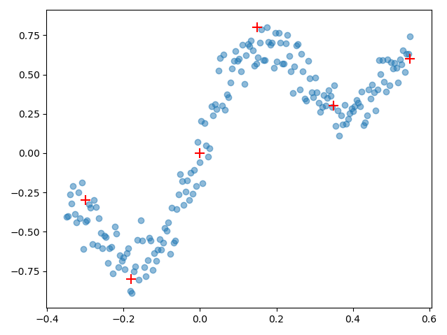
Judging from the regression data, we can see that the function which is represented by the noisy data points can be approximated quite reasonably with 6 data points. And this is what inducing points are all about: finding a set of representative points $\{ \widetilde{X}, \widetilde{y} \} $ which capture the original data structure $\{ X, y \}$ sufficiently well while reducing the memory and computational cost of the GP. Remember that we went from 200 data points to 6 data points, ergo a memory cost of $\mathcal{O}(200^2) = \mathcal{O}(40000)$ to just $\mathcal{O}(6^2) = \mathcal{O}(36)$.
The training objective consists now of maximizing the probability of the training data under the distribution of the GP with the inducing points $\widetilde{\mathcal{D}} = \{ \widetilde{X}, \widetilde{y} \}$. Thus we have the following objective function \(\begin{align} \min_{\theta, \widetilde{\mathcal{D}}} -\log p(\mathcal{D};\theta, \widetilde{\mathcal{D}}) &= \min_{\theta, \widetilde{\mathcal{D}}} -\log p(y| X; \theta, \widetilde{\mathcal{D}}) \\ &= \min_{\theta, \widetilde{\mathcal{D}}} -\log \mathcal{N} \Big( \overbrace{ K_{X \widetilde{X}} ( K_{\widetilde{X}, \widetilde{X}} + \sigma^2 I)^{-1} y}^{\mu(X)},\overbrace{ K_{XX} - K_{X \widetilde{X}} (K_{\widetilde{X} \widetilde{X}} + \sigma^2 I)^{-1} K_{\widetilde{X} X} + \sigma^2 I }^{\Sigma(X)} \Big) \end{align}\)
So let’s code that down in PyTorch!
So we already have the data. Next up is the base class for the GP. The most straight-forward way of using inducing points is to simply declare them as parameters which have gradients. Remember that both the objective function via the logarithm of the Normal distribution as well as the predictions consist of linear terms, so we can easily backpropagate through these operations to obtain the gradients for the kernel parameters and inducing points from the log probability of the true data under the Normal distribution of the GP.
class GP_InducingPoints(torch.nn.Module):

	def __init__(self, _x=None, _y=None, _num_inducing_points = params.num_inducing_points, _dim=1):

		super().__init__()

		assert type(_x) != type(None) # some sanity checking
		assert type(_y) != type(None) # some sanity checking for the correct input

		self.x = _x # save data set for convenience sake, not recommended for large data sets
		self.y = _y

		self.num_inducing_points = _num_inducing_points

		inducing_x = torch.linspace(_x.min().item(), _x.max().item(), self.num_inducing_points).reshape(-1,1) 	# distribute the data points as a linspace between x.min() and x.max() to get a good initialization of the inducing points
		self.inducing_x_mu = torch.nn.Parameter(inducing_x + torch.randn_like(inducing_x).clamp(-0.1,0.1)) 			# add some noise to the x values of the inducing points
		self.inducing_y_mu = torch.nn.Parameter(FloatTensor(_num_inducing_points, _dim).uniform_(-0.5,0.5)) 		# since we normalized the data to N(0,1) we initialize the y values in the middle of N(0,1)

		self.length_scale = torch.nn.Parameter(torch.scalar_tensor(0.1)) 	# the kernel hyperparameter to be optimized alongside inducing points
		self.noise = torch.nn.Parameter(torch.scalar_tensor(0.5)) 				# the noise hyperparameter to model the inherent variance in the data
Now we need the kernel method to compute the kernel/covariance matrix between arbitrary points:
	def compute_kernel_matrix(self, x1, x2):

			assert x1.shape[1] == x2.shape[1] # check dimension
			assert x1.numel() >= 0 # sanity check
			assert x2.numel() >= 0 # sanity check

			pdist = ( x1 - x2.T)**2 # outer difference
			kernel_matrix = torch.exp(-0.5*1/(self.length_scale+0.001)*pdist)

			return kernel_matrix
The third class method of the GP class to implement is the forward method of the GP such that we can take the gradients through PyTorch AutoDiff library:
	def forward(self, _X):

			# compute all the kernel matrices
			self.K_XsX = self.compute_kernel_matrix(_X, self.inducing_x_mu)
			self.K_XX = self.compute_kernel_matrix(self.inducing_x_mu, self.inducing_x_mu)
			self.K_XsXs = self.compute_kernel_matrix(_X, _X)

			# invert K_XX and regularizing it for numerical stability
			self.K_XX_inv = torch.inverse(self.K_XX + 1e-10*torch.eye(self.K_XX.shape[0]))

			#compute mean and covariance for forward prediction
			mu = self.K_XsX @ self.K_XX_inv @ self.inducing_y_mu
			sigma = self.K_XsXs - self.K_XsX @ self.K_XX_inv @ self.K_XsX.T + self.noise*torch.eye(self.K_XsXs.shape[0])

			# for each point in _X output MAP estimate and variance of prediction ( that's the torch.diag (...) )
			return mu, torch.diag(sigma)[:, None]
Up next is the loss function as described above:
	def NMLL(self, _X, _y):

			# set reasonable constraints on the optimizable parameters
			self.length_scale.data   = self.length_scale.data.clamp( 0.00001, 3.0)
			self.noise.data          = self.noise.data.clamp(0.000001,3)

			# compute all the kernel matrices again ... now you see why we want to use inducing points
			K_XsXs = self.compute_kernel_matrix(_X, _X)
			K_XsX = self.compute_kernel_matrix(_X, self.inducing_x_mu)
			K_XX = self.compute_kernel_matrix(self.inducing_x_mu, self.inducing_x_mu)
			K_XX_inv = torch.inverse(K_XX + 1e-10*torch.eye(K_XX.shape[0]))

			Q_XX = K_XsXs - K_XsX @ K_XX_inv @ K_XsX.T

			# compute mean and covariance and GP distribution itself
			mu = K_XsX @ K_XX_inv @ self.inducing_y_mu
			Sigma = Q_XX + self.noise**2*torch.eye(Q_XX.shape[0]) # noise regularized covariance

			p_y = MultivariateNormal(mu.squeeze(), covariance_matrix=Sigma)
			mll = p_y.log_prob(_y.squeeze()) # evaluate the probability of the target values in the training data set under the distribution of the GP

			mll -= 1/( 2 * self.noise**2) * torch.trace(Q_XX) # add a regularization term to regularize variance

			return -mll
And finally a nice plotting function:
	def plot(self, _title=""):

			x = torch.linspace(self.x.min()*1.5, self.x.max()*1.5, 200).reshape(-1,1)

			with torch.no_grad():
				mu, sigma = self.forward(x)

			x = x.numpy().squeeze()
			mu = mu.numpy().squeeze()
			sigma = sigma.numpy().squeeze()

			plt.title(_title)
			plt.scatter(self.inducing_x_mu.detach().numpy(), self.inducing_y_mu.detach().numpy())
			plt.scatter(self.x.detach().numpy(), self.y.detach().numpy(), alpha=0.1, c='r')
			plt.fill_between(x, mu-3*sigma, mu+3*sigma, alpha = 0.1, color='blue')
			plt.plot(x, mu)
			plt.xlim(self.x.min()*1.5, self.x.max()*1.5)
			plt.ylim(-3,3)
			plt.show()
Now we can let the whole thing train via the following script:
# generating data and normalizing it
X, y = generate_weightuncertainty_data()
X = FloatTensor(scale(X))
y = FloatTensor(scale(y))

# initialize the GP and plot initial prediction
gp = GP_InducingPoints(_x=X, _y=y)
gp.plot(_title="Init")

# use two different learning rates since inducing points need to potentially cover a far larger distance than kernel parameters
optim = torch.optim.Adam([{"params": [gp.length_scale, gp.noise], "lr": params.lr_kernel},
                          {"params": [gp.inducing_x_mu, gp.inducing_y_mu,], "lr": params.lr_ip}])

# put it all in a data loader ...
train_loader = DataLoader(TensorDataset(FloatTensor(X), FloatTensor(y)),
                        batch_size=params.num_samples,
                        shuffle=True,
                        num_workers=1)

# ... and let it train
for epoch in range(params.num_epochs):
	for i, (data, label) in enumerate(train_loader):
		optim.zero_grad()

		mll = gp.NMLL(data, label)

		mll.backward()
		optim.step()

		if epoch%(params.num_epochs//10)==0:
			print(f'Epoch: {epoch} \t NMLL:{mll:.2f} \t LS {gp.length_scale:.2f} \t Noise: {gp.noise:.2f}')
			gp.plot(_title=f"Training Epoch {epoch:.0f}")

gp.plot(_title="Post Training")
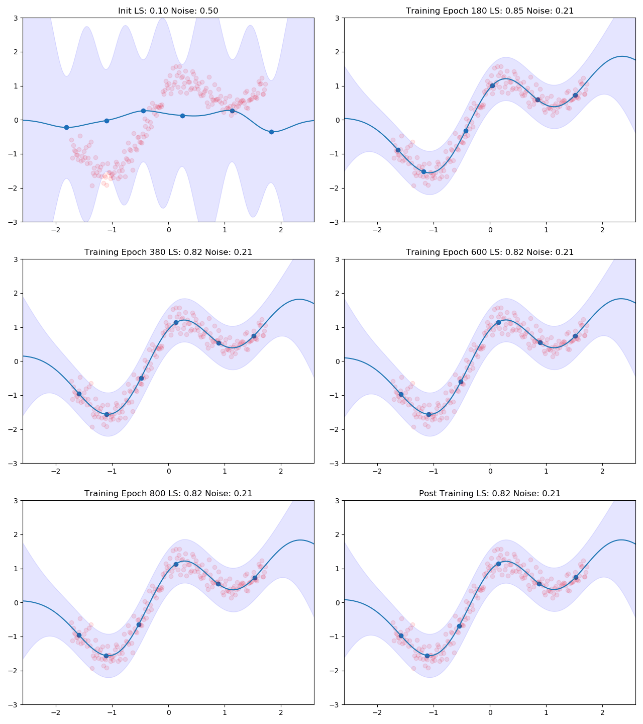
I combined the entire training loop into a nice little gif which shows how the inducing points and the kernel parameters are adjusted to the data:

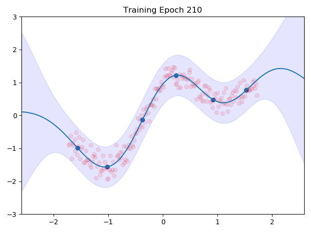
One can see nicely how the inducing points are moved to precisely the points in space which we predicted earlier in the image at the top. This training routine would even be amenable to mini batch training, we would introduce more variance though.