Hamiltonian Mechanics in Monte Carlo Samplers

Here’s a common problem: You want to estimate some function $f$. The function $f$ takes some input $x$ and outputs some value $y$ thus giving you $y=f(x)$. The important part is that you don’t have access to the global shape of $f$.

This could be due to $f(x)$ being an absolute black-box model such that you can only interact with it by handing it some value $x$ and receiving some value $y=f(x)$. Something that is practically very similar is that the analytical form of $f(x)$ is very, very complicated but can be evaluated in a pointwise manner. This means that we can’t evaluate the global shape of $f(x)$ but only the single points for some specific value of $x$.

The lack of knowledge of the global shape can be encountered in different scenarios which all boil down to computing a complicated integral. In order to offer some intuition let’s have a look at the univariate normal distribution $p(x|\mu, \sigma)$:

The univariate normal distribution is a true and tested distribution in machine learning with many convenient mathematical properties. One property is the normalization of the exponential term $\smash{e^{-\frac{(x-\mu)^2}{2\sigma^2}}}$ with the scaling term $1/\sqrt{2\pi\sigma^2}$ such that

Conversely we know that

Obviously we know the exact form of the scaling parameter through the standard deviation $\sigma$ … but what if we didn’t?

In that case we would encounter the distribution as

In the case above we could evaluate the distribution $p(x | \mu, \sigma)$ correctly up to the scaling parameter $1/Z$ by evaluating $f(x | \mu, \sigma)$. The value of $Z$ is given by the shape of the distribution $p(x | \mu, \sigma)$ which we can’t determine globally but only point-wise for some value $x$.

The example above is supposed to illustrate the more general problem of estimating probability distributions with intractable partition functions $Z$ while still being intuitive by working with a well known distribution such as the univariate normal distribution.

The most naive idea for computing $Z$ is to evaluate random values of $x$ and compute an approximate integral. More precisely we would sample $N$ different $x$ from a uniform distribution $U(x_{min}, x_{max})$ with equal probability. This set $\{ x_i \}_{i=0}^N$ serves as an approximation of the true function which becomes better and better, the more samples $x_i$ we obtain. If we were to choose $N=\infty$ then the sample set would replicate the true shape perfectly. This is practically impossible due to computational and time constraints.

Once we have a set which we think contains enough samples, we could approximate the integral by simply summing over our set

The $\Delta x$ is required since are we approximating the function $f( x | \mu, \sigma)$ with little columns where the exponential term tells us the height and $\Delta x$ the width of the column (look at the animations at Wikipedias entry for Riemann integral).

This would get the job done as our approximation would asymptotically approach the true value of $Z$ for large enough sample sizes. Yet, upon closer examination we can see that the univariate normal distribution has a specific shape which concentrates a lot of information (or more precisely probability) in the area around $\mu$.

Remember that a the bulk of the integral $\smash{\int_{-\infty}^{\infty} f(x|\mu, \sigma) dx}$ is evaluated around $\mu$. If we chose $x_{min}$ and $x_{max}$ at the very extreme ends of the number line, our $N$ samples would be very dispersed and our approximation of $Z$ would be very poor.

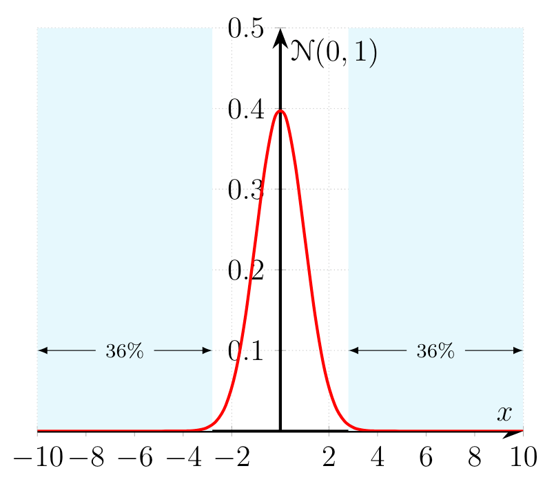
Let’s examine a concrete problem. We choose a standard normal distribution $\mathcal{N}(0,1)$ and sample $200$ values of $x$ from the uniform distribution $\mathcal{U}(-10,10)$. Furthermore we consider all probabilities of $\mathcal{N}(0,1)$ interesting which have a probability above $p(x|\mu, \sigma) \geq 0.01$.

print()
print('###########################################')
print('Uniform Sampler')
print('###########################################')

import numpy
import numpy as np
import scipy as sp
import matplotlib.pyplot as plt
import torch
import math

FloatTensor = torch.FloatTensor

class Gaussian:

	def __init__(self, _mu, _sigma):
		self.mu = _mu
		self.std = _sigma
		self.dist = torch.distributions.Normal(self.mu, self.std)

	def eval(self, _x):
		return self.dist.log_prob(_x).exp()

	def unnorm_eval(self, _x):
		return torch.exp(-1/(2*self.std**2)*(_x - self.mu)**2)
std = 1
print('True Z:', np.sqrt(2*np.pi*std**2))
P = Gaussian(FloatTensor([0]), FloatTensor([std]))
U = torch.distributions.Uniform(0,1)
num_samples=1000

res = 100
x_min=-10
x_max=10
points = torch.from_numpy(np.linspace(x_min,x_max,res))
probs = FloatTensor([P.eval(point) for point in points])

plt.figure(figsize=(10,10))
plt.plot(points.numpy(), probs.numpy())
sample_points = torch.distributions.Uniform(x_min, x_max).sample((num_samples,))
sample_probs = FloatTensor([P.unnorm_eval(point) for point in sample_points])

# Compute Z
Z = sample_probs.sum()/(num_samples/(x_max - x_min))
sample_probs /= Z
print('Estimated Z:', Z.numpy())

print('1D Uniform Sampler: P(x)>=0.01: ', sample_probs[sample_probs>=0.01].shape[0]/sample_points.shape[0]*100, '%')

plt.scatter(sample_points.numpy(), sample_probs.numpy())
plt.show()

###########################################
Uniform Sampler
###########################################
True Z: 2.5066282746310002
Estimated Z: 2.5824146
1D Uniform Sampler: P(x)>=0.01:  26.1 %

As it turns out $ \approx 74\%$ of the values $x \in [-10,10]$ are below $0.01$. That means that by sampling randomly from a uniform distribution $\mathcal{U}(-10,10)$ we would evaluate $72\%$ of our randomly selected values $x$ with a probability below $0.01$ thus effectively wasting a large number of samples. Conversely only $28\%$ of the samples would lie in probability regions around the mean $\mu$ with a probability higher than $0.01$. The evaluation of the area close to $\mu$ would therefore be highly inefficient as we waste a considerable amount of samples in areas which do not contribute to the integral of $Z$.

Obviously we could restrict the uniform distribution $\mathcal{U}(x_{min}, x_{max})$ to be closer to the value of $\mu$ but this could only be efficiently be done if we were to have specific prior information about the distribution. Similarly, the area with probabilities below 0.01 decreases if we increase the variance of the Normal distribution. Again, this is just a toy example to visualize the problems when sampling from high-dimensional spaces. The main take way point is that one has to pay close attention to what the sampler is doing and how sampling algorithms are designed to make efficient use of computational resources. I’ll get into the geometric details of high dimensional spaces later.

Can we do any better? … In fact we can with the help of physicists from the Manhattan Project and a chain.

In the example above we want to sample as often as possible in the areas which greatly contribute to the integral $Z = \int_{-\infty}^{\infty} f(x|\mu, \sigma) dx$. So we could say that once we happen to sample close to $\mu$ we would like to sample as often as possible in the same area, effectively staying in the area around $\mu$.

The achievement of Mr Metropolis et al. and the extensions by Mr Hastings (is the Netflix-Founder related to him?) was to elaborate precisely that idea and introduce the concept of a sampling chain to our problem.

The sampling chain is a sequence of samples ${x_0, x_1, \ldots, x_N}$ which is constructed iteratively by sampling a proposal point $x_t’$ and accepting it as the next sample $x_{t+1}$ based on an acceptance condition. The proposal sample $x’_t$ can be be rejected and in that case a new proposal sample $x’_t$ has to be proposed. The important part is how the proposed samples in the chain are generated, accepted and rejected.

In order to stay in areas which contribute to the value of Z, we can propose a sample $x’_t$ which is close to our current sample $x_t$ and evaluate $f(x’_t|\mu, \sigma)$. We can then compare the new evaluated sample $f(x’_t|\mu, \sigma)$ and the current evaluated sample $f(x_t|\mu, \sigma)$ and accept the proposed sample $x’_t$ as the next sample if $f(x’_t|\mu, \sigma) \geq f(x|\mu, \sigma)$.

Before long the straight-forward acceptance rule $f(x’_t|\mu, \sigma) \geq f(x_t|\mu, \sigma)$ would take us straight to $x = \mu$. The problem is that we would be stuck in $x = \mu$ as every value $x \neq \mu$ has a lower evaluation $f(x\neq\mu |\mu, \sigma)$ than $f(x = \mu|\mu, \sigma)$. You can verify that by simply looking at a plot of a normal distribution.

In order to stay in the high value area around $\mu$ but also not get stuck in it, a proposal distribution $q(x’|x)$ is evaluated, the ratio $f(x’_t|\mu, \sigma)/f(x_t|\mu, \sigma)$ is used which is then compared to an auxiliary sample: $U \sim \mathcal{U}(0,1)$. This is done in the following way:

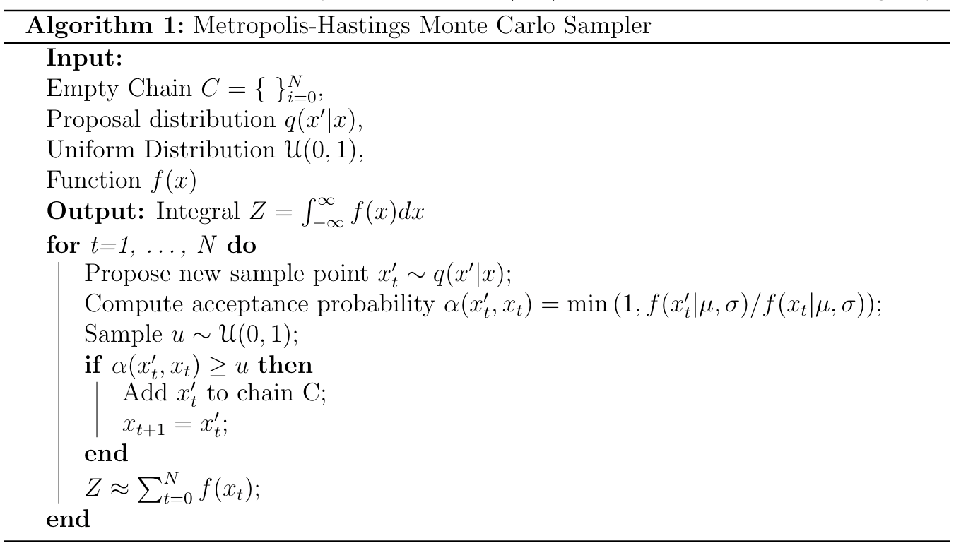
The acceptance ratio $\alpha$ is computed in a smart way, namely that $f(x’_t|\mu, \sigma)/f(x_t|\mu, \sigma) \in (0,\infty)$. If $f(x’_t|\mu, \sigma)$ is larger than $f(x_t|\mu, \sigma)$, then $f(x’_t|\mu, \sigma)/f(x_t|\mu, \sigma) \geq 1$ and the proposal sample will always be accepted. If on the other hand $f(x’_t|\mu, \sigma) \leq f(x_t|\mu, \sigma)$, then $f(x’_t|\mu, \sigma)/f(x_t|\mu, \sigma) \in (0,1)$ there is a chance that we accept the proposed sample $x’_t$ anyway if $u > \alpha$. By sampling $u \sim \mathcal{U}(0,1)$, occasional steps into areas with lower values $f(x)$ are allowed.

The final component is the proposal distribution $q(x’|x)$ which is chosen in its simplest form as a standard normal distribution around $x$, namely $x’ \sim \mathcal{N}(x, 1)$. The chain $\{ x_t \}_ { i=0 }^N$ that is constructed during sampling exhibits the Markov property such that each state $x_t$ is only dependent on the previous state $x_{t-1}$ through the proposal distribution $q(x’|x)$ (and after the proposal was accepted). The Markov chain property and the Monte Carlo sampling process together define the broader class of sampling algorithms called ‘Markov Chain Monte Carlo’ (MCMC).

An important criterion while constructing such a Markovian chain of samples is that the sampler can move through the state space in an unbiased way. The acceptance probability and the proposal distribution should therefore guarantee that the sampler can reach every state if we sample long enough. For the Metropolis-Hastings algorithm it is required that the proposal density is symmetric such that $q(x’|x) = q(x|x’)$. This can be realized easily with a Normal distribution with constant standard deviation. Mathematically, it is required that the Markov chain is reversible which simply states that there should be equal probability when being in state $x$ and moving to $x’$ and reverse:

We can now decompose the transition probability $ p(x’|x) $ into the proposal distribution $q(x’|x)$ and the acceptance probability $\alpha(x’|x)$:

The equation above simply states that the probability of being in state $x$, proposing to go to state $x’$ and finally accepting to go the state $x’$ should be the same as doing the three steps in reverse. This guarantees that no state $x$ is favored in any particular way and that the final Markov chain asymptotically approaches the true value of $Z$.

We can now plug in the acceptance probability of the Metropolis-Hastings sampler and pull the transition and stationary probabilities into the minimum operator:

The above equation is valid and states that the ‘detailed balance’ property holds for the acceptance ratio of the Metropolis-Hastings sampler. Thus in statistical lingo, we have an unbiased estimator of the true $Z$ which will asymptotically approach the true of value of $Z$!

	print()
	print('###########################################')
	print('Metropolis-Hastings')
	print('###########################################')


	import numpy
	import numpy as np
	import scipy as sp
	import matplotlib.pyplot as plt
	import torch
	import math

	FloatTensor = torch.FloatTensor

	class Gaussian:

		def __init__(self, _mu, _sigma):
			self.mu = _mu
			self.std = _sigma
			self.dist = torch.distributions.Normal(self.mu, self.std)

		def eval(self, _x):
			return self.dist.log_prob(_x).exp()

		def unnorm_eval(self, _x):
			return torch.exp(-1/(2*self.std**2)*(_x - self.mu)**2)

	std = 1
	print('True Z:', np.sqrt(2*np.pi*std**2))
	P = Gaussian(FloatTensor([0]), FloatTensor([std]))
	Q = torch.distributions.Normal(FloatTensor([0]), FloatTensor([1]))
	U = torch.distributions.Uniform(0,1)
	num_samples=100

	res = 200
	x_min=-10
	x_max=10

	#Deterministic evaluation for plotting purposes
	points = torch.from_numpy(np.linspace(x_min,x_max,res))
	probs = FloatTensor([P.eval(point) for point in points])
	plt.figure(figsize=(10,10))
	plt.plot(points.numpy(), probs.numpy())

	# Initialize starting point of chain randomly in U(-10,10)
	x_init = torch.distributions.Uniform(x_min, x_max).sample((1,))
	x = x_init

	accepted_x = []
	accepted_y = []
	rejected_x = []

	num_samples=1000
	burn_in = 200 # Burn_in to make up for random initialization
	for i in range(num_samples+burn_in):

		x_ = Q.sample()
		a = P.unnorm_eval(x+x_)/P.unnorm_eval(x)
		if a >= U.sample():
			if i >= burn_in:
				accepted_x.append(x+x_)
				accepted_y.append(P.unnorm_eval(x+x_))
			x = x+ x_
		else:
			if i >= burn_in: rejected_x.append(x+x_)

	accepted_x = torch.stack(accepted_x, dim=0)
	accepted_y = torch.stack(accepted_y, dim=0)
	rejected_x = torch.stack(rejected_x, dim=0)
	print('Accepted/Rejected: ', accepted_x.shape[0], '/', rejected_x.shape[0])

	#Computing Z
	num_bins = 200
	bins = np.linspace(x_min, x_max, num_bins)
	index = np.digitize(accepted_x, bins)


	bin_counts = np.array([np.sum([index == i]) for i in range(1, len(bins))])
	bin_y_sums = np.array([accepted_y.numpy()[index == i].sum() for i in range(1, len(bins))])

	tmp = bin_y_sums/bin_counts
	tmp[np.isnan(tmp)]=0

	print('Estimated Z:', sum(tmp)/(num_bins/(x_max-x_min)))

	accepted_probs = FloatTensor([P.eval(point) for point in accepted_x])
	print('1D MH Sampler: P(x)>=0.01: ', accepted_probs[accepted_probs>=0.01].shape[0]/num_samples*100, '%')

	plt.scatter(accepted_x.numpy(), accepted_probs.numpy())
	plt.show()

	###########################################
	Metropolis-Hastings
	###########################################
	True Z: 2.5066282746310002
	Accepted/Rejected:  701 / 299
	Estimated Z: 2.4467572424682826
	1D MH Sampler: P(x)>=0.01:  69.69999999999999 %

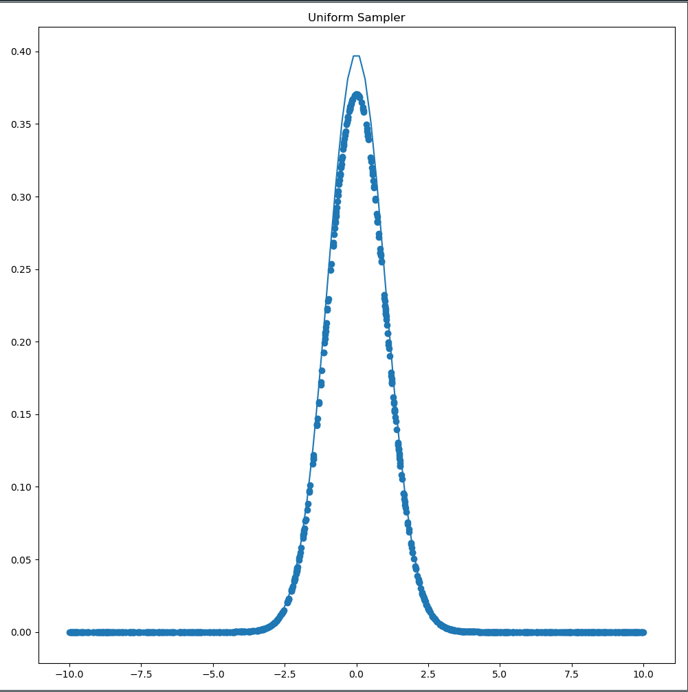
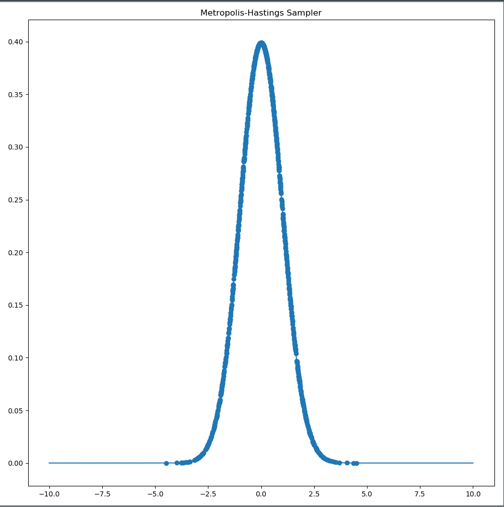
The uniform sampled used $26 \%$ of its samples in useful areas whereas the Metropolis-Hastings sampler uses almost $70 \%$! We can visualize the two samplers next to each other to visualize the increased efficiency of the Metropolis-Hastings Sampler.

We can even visualize a Metropolis-Hastings sampler in two dimensions with the accepted and rejected samples:

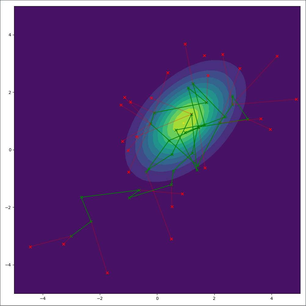
It’s observable how moves closer to the center of the probability distribution are always accepted whereas moves away are sometimes accepted. In the cases where the proposed sample is in significantly lower value areas, the move will be rejected.

We can even improve our sampler even further by treating the surface of the distribution as a physical model. In order to illustrate we should first take the $-\log$ of the unnormalized function $f(x|\mu, \sigma)$:

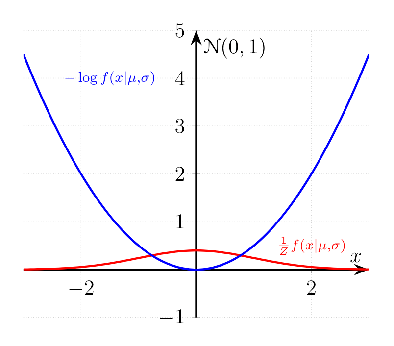
By working with $-\log f(x | \mu, \sigma)$ we get rid of the pesky exponential term, effectively working with a linear function in case of the Normal distribution. Additionally, we have transformed the function $f(x|\mu, \sigma)$ into a nice representation where the bottom of the curve $-\log f(x|\mu, \sigma)$ represents the areas in $f(x|\mu, \sigma)/Z$ with the highest probabilities.

Remember that the Metropolis-Hastings sampler was developed by the physicists at the Manhattan Project to tackle the problem in statistical mechanics of estimating the partition function $Z$. In statistical mechanics, the function $f(x)$ is the energy function $E(x)$ of a system in state $x$ and the probability of the system being in state $x$ is defined by

The probability of a system being in state $x$ increases if the energy of that state $x$ is small. This corresponds to the basic physical behavior, that physical systems want to be in a minimal energy state. If a piece of metal is hot, it emanates heat and cools down and decreases its energy. If a ball has high potential energy, it will decrease this energy by dropping down. If a coil is being compressed, it will expand once the force relents to enter into a low energy state.

We will now introduce a second idea from physics: Hamiltonian Mechanics. Let’s say you have physical system $\mathcal{H}(x, p, t)$ in which two properties describes everything you know. These two properties are the position $x(t)$ and the momentum $p(t)$. For some position $x(0)$ and the momentum $p(0)$, the physical system $\mathcal{H}(x, p, t)$ will be able to predict every future position $x(t)$ and momentum $p(t)$.

This is possible due to the following Hamiltonian mechanics:

The Hamiltonian $\mathcal{H}(x, p, t)$ corresponds in our simple case to the energy of the system. The two differential equations above describes how the energy of the system is allocated to either the momentum $p(t)$ or the position $x(t)$ as time progresses.

The energy of the system $\mathcal{H}(x, p, t)$ consists of the potential energy $E_p(x(t))$ and the kinetic energy $E_k(p(t)) = p(t)^2/2m$ for a particle of mass $m$: \(\begin{align*} \mathcal{H}(x, p, t) = E_p(x(t)) + E_k(p(t)) = E_p(x(t)) + \frac{p(t)^2}{2m} \end{align*}\)

We can apply the Hamiltonian mechanics from above to our function $-\log f(x | \mu ,\sigma)$ and simulate the trajectory of a particle with $m=1$. For that to happen we first derive both $dp(t)/dt$ and $dx(t)/dt$ for the potential energy provided by $ E_p(x(t)) = - \log f(x(t) | \mu, \sigma)$:

We can now use the derivations above to simulate the trajectory of a particle on the surface of $-\log f(x(t) | \mu, \sigma)$ applying the following update steps to the position $x(t)$ and momentum $p(t)$ of the particle:

These two update rules have very intuitive explanations once we have look at the shape of $-\log f(x(t) | \mu, \sigma)$:

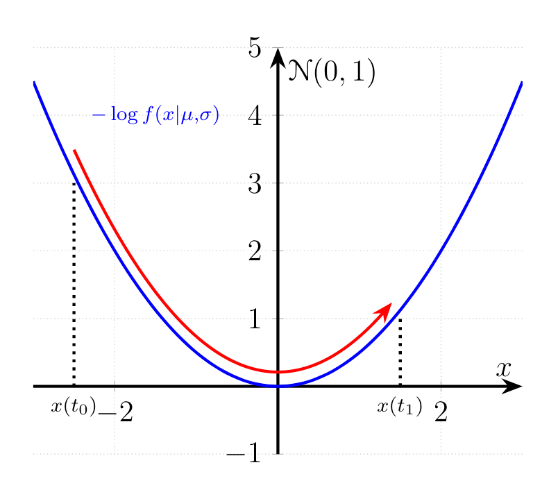
The particle starts at $x(t_0)$ with a high potential energy and some initial momentum $p(t_0)$. The gradient of $-\log f(x(t_0)|\mu, \sigma)$ is very steep and thus a lot of extra momentum is added to the particles kinetic energy. The direction of steepest descent $-\partial \log f(x(t)|\mu, \sigma)/dx(t)$ points in the negative direction on the x-axis and thus extra momentum is added due to the minus sign. The potential energy $-\log f(x(t)|\mu, \sigma)$ decreases as the particle moves to the lower area. Once the particle moved past $x(t)=0$ the trend reverses and the gradient $\partial \log f(x(t)|\mu, \sigma)/dx(t)$ is positive, thus decreasing the momentum.

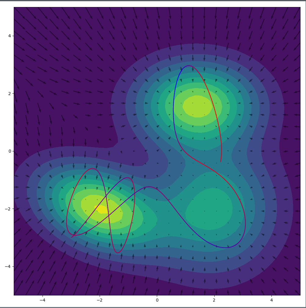
While the one dimensional case above is nice to gain an intuition, this whole simulation looks significantly cooler in two dimensions. I plotted the $- \log f(x(t)|\mu, \sigma)$ surface with the resulting gradients of the surface as arrows. We can see nicely how the particle runs up the slope at the edge of the low energy basins. After all its momentum has been converted into potential energy, it makes a u-turn and heads back down the slope. (That’s actually something we want to prevent which lead to the development of the No-U-Turn-Sampler (NUTS)).

Here’s some code with PyTorch:

	import numpy as np
	import matplotlib
	import matplotlib.pyplot as plt
	import torch

	FloatTensor = torch.FloatTensor

	pi = FloatTensor([np.pi])


	class Potential:

		#GMM with three different clusters
		def __init__(self):
			self.mean1 = FloatTensor([-2, -2])
			self.covar1 = FloatTensor([[2, -0.5],[-0.5, 1]])
			self.mean2 = FloatTensor([1.4, 1.6])
			self.covar2 = FloatTensor([[2, 0],[0, 1]])
			self.mean3 = FloatTensor([2, -2])
			self.covar3 = FloatTensor([[2, 0],[0, 2]])

		def log_eval(self, x):

			dist1 = torch.distributions.MultivariateNormal(self.mean1, self.covar1)
			dist2 = torch.distributions.MultivariateNormal(self.mean2, self.covar2)
			dist3 = torch.distributions.MultivariateNormal(self.mean3, self.covar3)

			return torch.log(1/3*torch.exp(dist1.log_prob(x))
					 + 1/3*torch.exp(dist2.log_prob(x))
					 +1/3*torch.exp(dist3.log_prob(x)))

	#Initialize potential
	potential = Potential()

	#Data for plotting the surface  
	res = 50
	x = np.linspace(-5,5,res)
	y = np.linspace(-5,5,res)
	X,Y = np.meshgrid(x, y)
	points = FloatTensor(np.stack((X.ravel(),Y.ravel())).T).requires_grad_()
	probs = FloatTensor([potential.log_eval(point).exp() for point in points]).view(res,res)

	#Data for plotting the gradients
	res_coarse = 25
	x_coarse = np.linspace(-5, 5, res_coarse)
	y_coarse = np.linspace(-5, 5, res_coarse)
	X_coarse,Y_coarse = np.meshgrid(x_coarse, y_coarse)
	points_coarse = FloatTensor(np.stack((X_coarse.ravel(),Y_coarse.ravel())).T).requires_grad_()
	grads = [torch.autograd.grad(outputs=potential.log_eval(point), inputs=point)[0] for point in points_coarse]
	grads = torch.stack(grads, dim=0).numpy()

	#Plotting both surface and gradients
	plt.figure(figsize=(10,10))
	plt.contourf(X, Y, probs.numpy(), levels=10)
	plt.quiver(X_coarse, Y_coarse, grads[:,0], grads[:,1], color='black', alpha=0.5)

	#The two lists store the trajectory data
	traj = []
	nuts_criterion = []

	#Initialize the starting position and momentum for the particle
	x = FloatTensor([-2,-2.5]).requires_grad_() # Position
	p = FloatTensor([1,0]) # Momentum

	for i in range(600):

		p = p + 0.05 * torch.autograd.grad(outputs=potential.log_eval(x), inputs=x)[0]
		x = x + 0.05 * p

		traj.append(x.detach())
		nuts_criterion.append((x - x_init).dot(p).detach())

	traj = torch.stack(traj, dim=0).numpy()
	nuts_criterion = torch.stack(nuts_criterion).numpy()
	nuts_criterion = (nuts_criterion-nuts_criterion.min())/(nuts_criterion.max() - nuts_criterion.min())

	for i in range(traj.shape[0]-1):
		plt.plot([traj[i,0], traj[i+1,0]], [traj[i,1],traj[i+1,1]], c=(1-nuts_criterion[i], 0, nuts_criterion[i]))

	plt.show()

The total energy of the particle is conserved between the potential and the momentum. We show this by initializing the particle with a very high potential energy and a high momentum and watch it slide over the surface of the distribution in wide arcs.

Alternatively we could initialize the particle with little potential energy and little momentum. Since the total energy of the particle is low, it will remain in the low energy (=high probability) basin and sample amply from there.

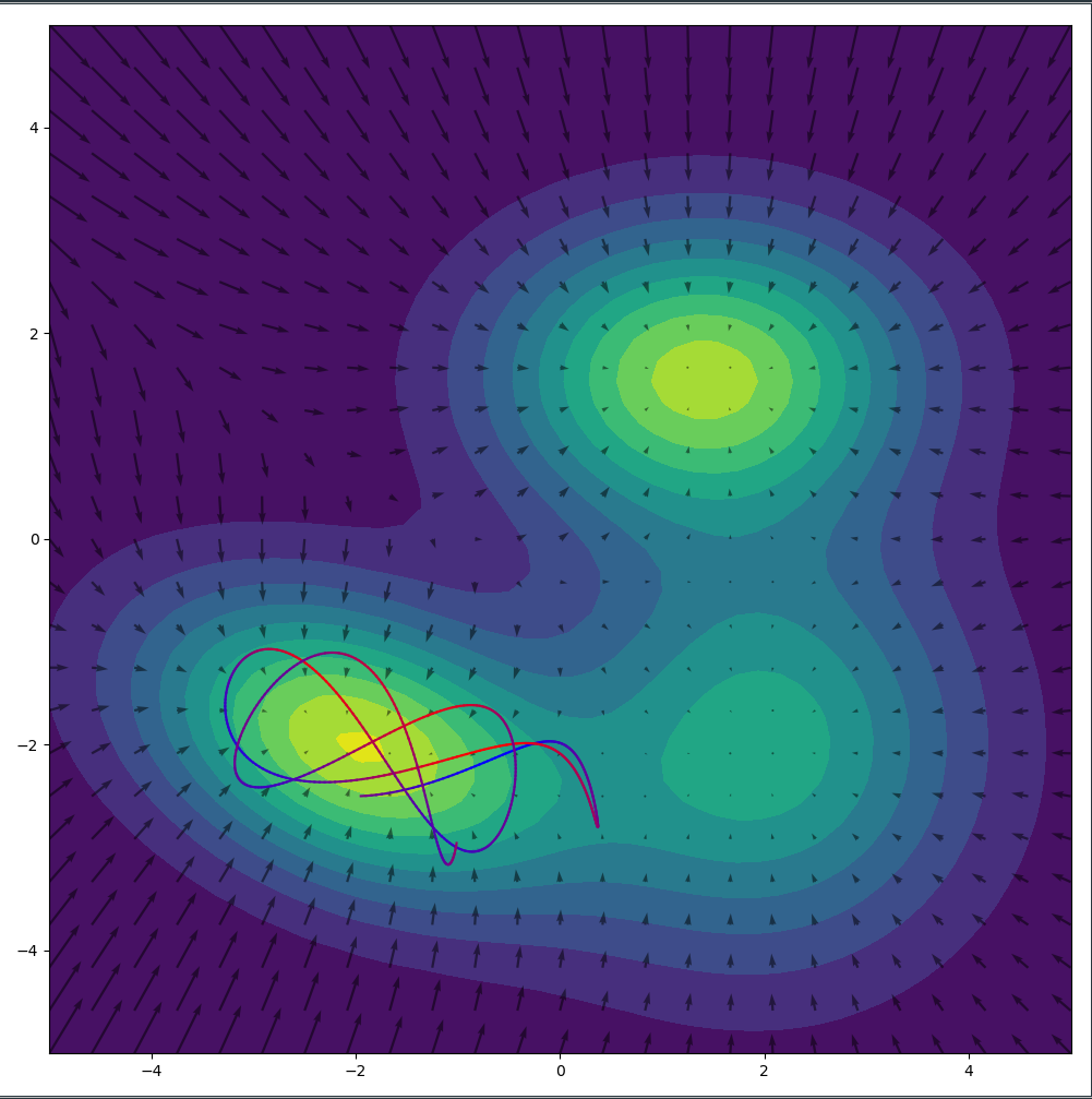
The total energy initialization of the particle at the start of each trajectory can be drawn from a distribution. The distribution can easily be incorporated into the detailed balance equation and marginalized out such that the sampler is unbiased.

Here are two links to fully implemented Hamiltonian Monte Carlo Samplers with crazy awesome animations: here and here

A closing remark about the geometry of high-dimensional spaces:

While sampling methods are asymptotically correct in their estimation of the posterior distribution, they do not scale well due to the curse of dimensionality. In a nutshell it refers to the geometric properties of high dimensional spaces. For example the distance between two points increases as we move into higher and higher dimensional spaces. A quick example is the Euclidean distance between two points which have a distance of 1 in every of their shared dimensions $\mathbb{R}^N$. Depending on the dimensionality $N$ we get a distance $\sqrt{\sum_{n=0}^N 1^2}$:

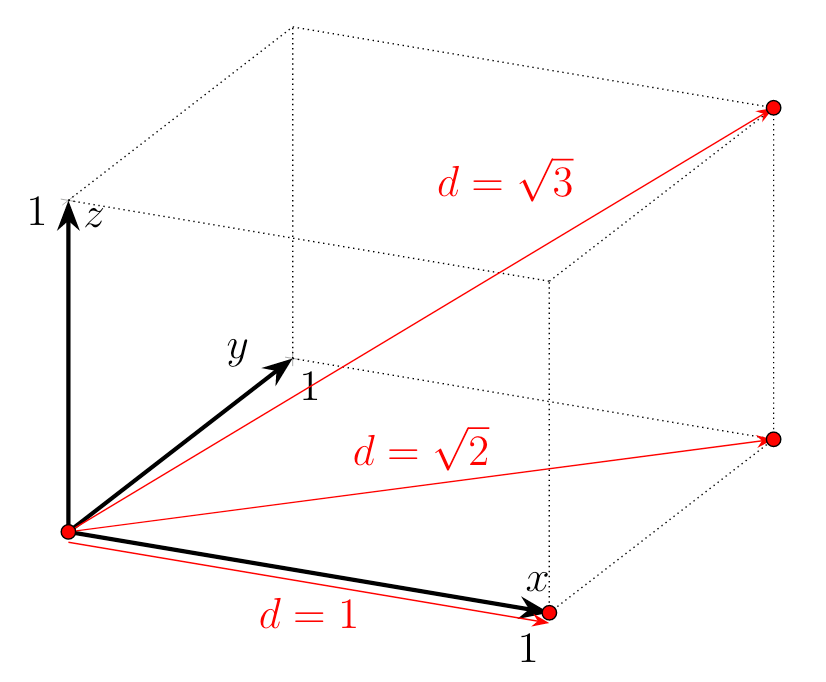
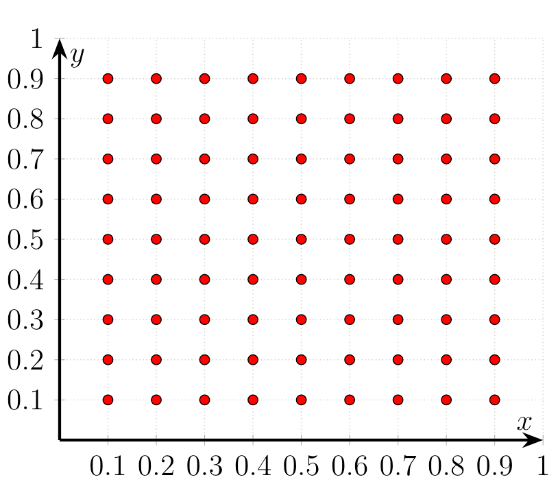
The more dimensions we add, the larger the space between two points with equal distance in every dimension. Secondly this creates the problem of requiring an increasing number of samples for higher and higher dimensional spaces. Let’s say we want to estimate a function by sampling in the Euclidean space spanned between two points with unit distance, ergo distance of 1. We want to estimate the function and want a resolution of 0.1, i.e. we need 10 samples per dimension. In $\mathbb{R}^1$ we only require 10 samples to estimate the pdf wit equally spaced sampling points.

But in $\mathbb{R}^2$ we suddenly require 100 samples to estimate the function with the desired resolution.

In $\mathbb{R}^3$ we finally need 1000 samples to estimate the function to our liking.

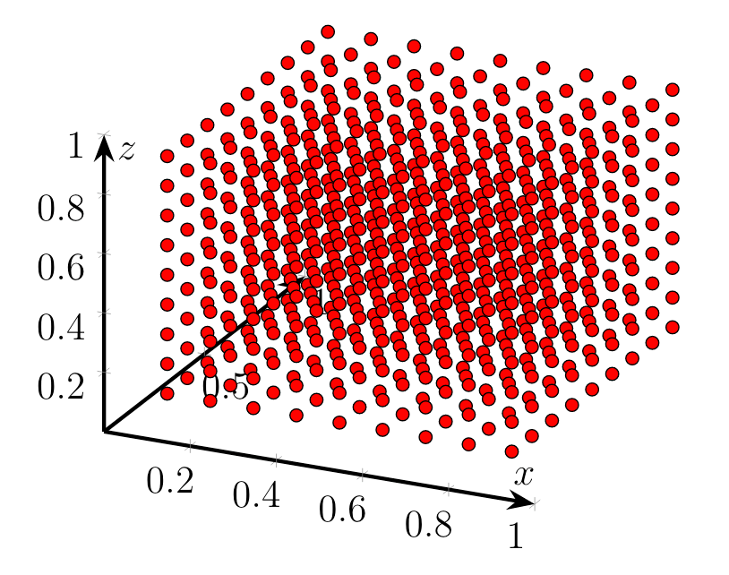
The required number of samples grows exponentially with the number of dimension, i.e. $10^N$ in $\mathbb{R}^N$ for our specific setup of 10 samples per dimension. By just adding two dimensions we need $100 \times$ more samples than in one dimension. That might not sound like a lot, but it quickly accumulates when working in high-dimensional spaces. This effectively restricts sampling algorithms to applications where we require very precise posteriors as in finance or medicine or where the run-time isn’t a problem.