Girsanov What?

I encountered Girsanov’s theorem repeatedly as I was reading stochastic processes paper and talking to people from that community.

A quick look at Wikipedia returned something that was absolute unintelligible to me (without a proper higher math education).

Thus began a chase down the rabbit whole for alternative sampling in stochastic processes. :-)

Importance Sampling

The first thing that I noticed was that the term \(\frac{dQ}{dP}\) occured in a lot of text books that I found on Google. In this context both $P$ and $Q$ are probability measures which assign a scalar value to whatever space they are assigned to. This ratio occurs often in what machine learners call importance sampling. Imagine you want to compute the average value of a random variable $X$ which follows a very complicated probability density function $p(x)$ which you can only evaluate and never sample from. Mathematically, you would be interested in $\mathbb{E}_{q(x)}[X] = \int x \cdot q(x) dx$.

Fundamentally, this expected value is an integral. For simple systems this integral might offer a way to compute it analytically, but for anything of relevant size an analytical solution is probably very, very hard to obtain. Imagine some highly complicated physical, chemical or biological system that on theoretical grounds follows some probability distribution but which is just really difficult to sample from.

This leaves us the numerical approach. In a grid based approach, we could take every value $x$, evaluate $p(x)$, multiply them and add them. Again, for small and simple systems that might be laborious but yield the correct value but is infeasible for relevant systems. Also, $x$ could be continuous so we would need by definition an infinite amount of samples as there are an infinite amount of values in any continuous range. This leaves us with the sampling approach in which we don’t take every value, but only a subset of size $N$ and literally hope that a finite number of samples will yield a sufficiently exact value. The sampling approximation would be

But we said earlier that sampling from $q(x)$ is not feasible. How do we reconcile this apparent contradiction? The answer to this is the simplest mathematical operation we can think of: a multiplication with $1$. Ah, and also we need a second easy probability distribution $p(x)$.

To see why let’s write out the expectation,

Now, if we write out this expectation in its sampling approximation we get

This approximation implies that we can compute the exact integral/expected value by sampling from an alternative distribution $p(x)$ and rescaling and multiplying it not with $q(x_i)$ but with the ratio $\frac{q(x_i)}{p(x_i)}$.

Intriguing …

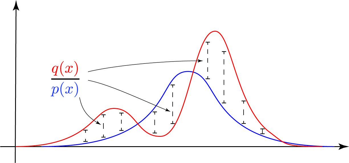
Let’s try to visualize whats happening. In the image below is a ‘complicated’ red distribution with two modes. To get the point across, we assume we can’t sample from it. Instead we take a blue Normal distribution and sample $x_i$ from it. Whenever a sample $x_i$ has higher probability under $p(x)$ than under $q(x)$, the ratio automatically decreases the contribution in the product $x_i \cdot \frac{q(x_i)}{p(x_i)}$ and vice versa. So the ratio of the two distributions serves as a sort of corrector for the ‘incorrect’ sampling. Nice.

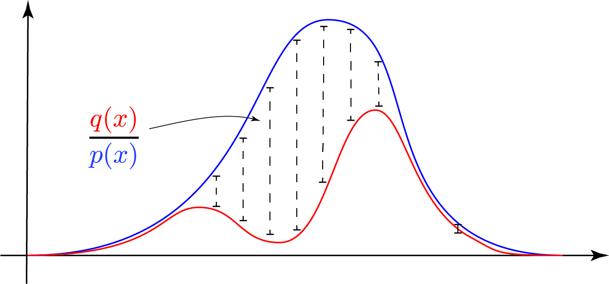
But the astute observer should observe a fundamental flaw in the left and right hand side of the figure above. Remember that we draw samples exclusively from the blue curve. Only in the central part is the blue curve actually ‘above’ the red curve. To the left and to the right, we are under-sampling the distribution. Whenever the blue proposal distribution has less probability than the target distribution, we’re missing out on potential action. As in life, the premise ‘Better safe than sorry’ holds here as well. A better blue proposal distribution would be:

Here, we cover every mode and only have to correct downward and we are not potentially undersampling certain modes as before.

‘Importance Sampling’ for Stochastic Processes

Let’s assume we have two stochastic processes ${X^p_t}$ and ${X^q_t}$,

where as $X^p_t$ is a pure Wiener process, the stochastic process $X^q_t$ exhibits both a drift as well as diffusion term.

Solving these two processes generates a probability distribution over space and time and both are said to be driven by an underlying source of randomness, in this case a Wiener process. They induce a probability measure $P$ and $Q$ and their respective probability density functions $p(x)$ and $q(x)$.

Next, would like to compute the expected value over some function of the realizations of the stochastic process $f({X^q_t})$,

Similar to above, it now turns out that actually sampling $X^q_t$ is very difficult. But fortunately for us, we can apply the intuition that we gained from the importance sampling approach and apply here as well.

Recall that $X^p_t$ is a pure Wiener process and thus the probability of a particular realization can be computed quite easily. This is due to the fact that in a Wiener proces, every movement is independently and identically distributed (iid).

To make things easier to show, we have to agree on a time discretization, which we will here choose as $\Delta t$. This means that we do $\Delta t$ steps in time. Concurrently, the process $X^p_t$ is now discretized into $\Delta t$ time steps as well.

From the analytical distribution of a Wiener process we can determine the probability of each step as

For a series of steps in a particular realization ${ x^p_{t_k} }$ of the stochastic process $X^p_t$, we would be interested in the total probability of that particular realization. Since each step in a Wiener process is independent, we factorize over the steps and get a multiplication of Gaussians,

Now we can do the same for the $Q$ process with the non-standard-Wiener process. Here, the discretization yields

where the probability of the next step is determined by Gaussian with the drift as the mean and the diffusion as the uncertainty. Thus large steps away from the predicted drift will naturally receive little probability whereas staying close to the drift will be of high probability.

We can equally compute the probability over an entire sequence by factorizing the individual steps,

Little else is left to arrive at Girsanov’s theorem than computing the ratio between these two probability distributions, since we can do importance sampling over stochastic processes via

Actually computing the ratio yields

Now we further simplify the upper of the fraction to get

We can plug that back in to obtain

Reverting the time discretization, we in fact see that these sums transform into integrals of the form,

And thus we arrive at the weighting factor \(\begin{align} \frac{q}{p}(x^p_{t_k}) \\ &= \exp \left(\int a_t dX_t - \frac{1}{2} \int a_t^2 dt \right) \end{align}\)

which will allow us to sample from a simple Wiener process $X^p_t$, and reweight it such that we’re actually correctly sampling from $X^q_t$:

The quantity $Z(X^p_t)$ allows us to sample pure Brownian motion $X^p_t$, evaluate it with $f(X^p_t)$ and reweight it correctly with $Z(X^p_t)$ within the expectation over $P$, not $Q$.

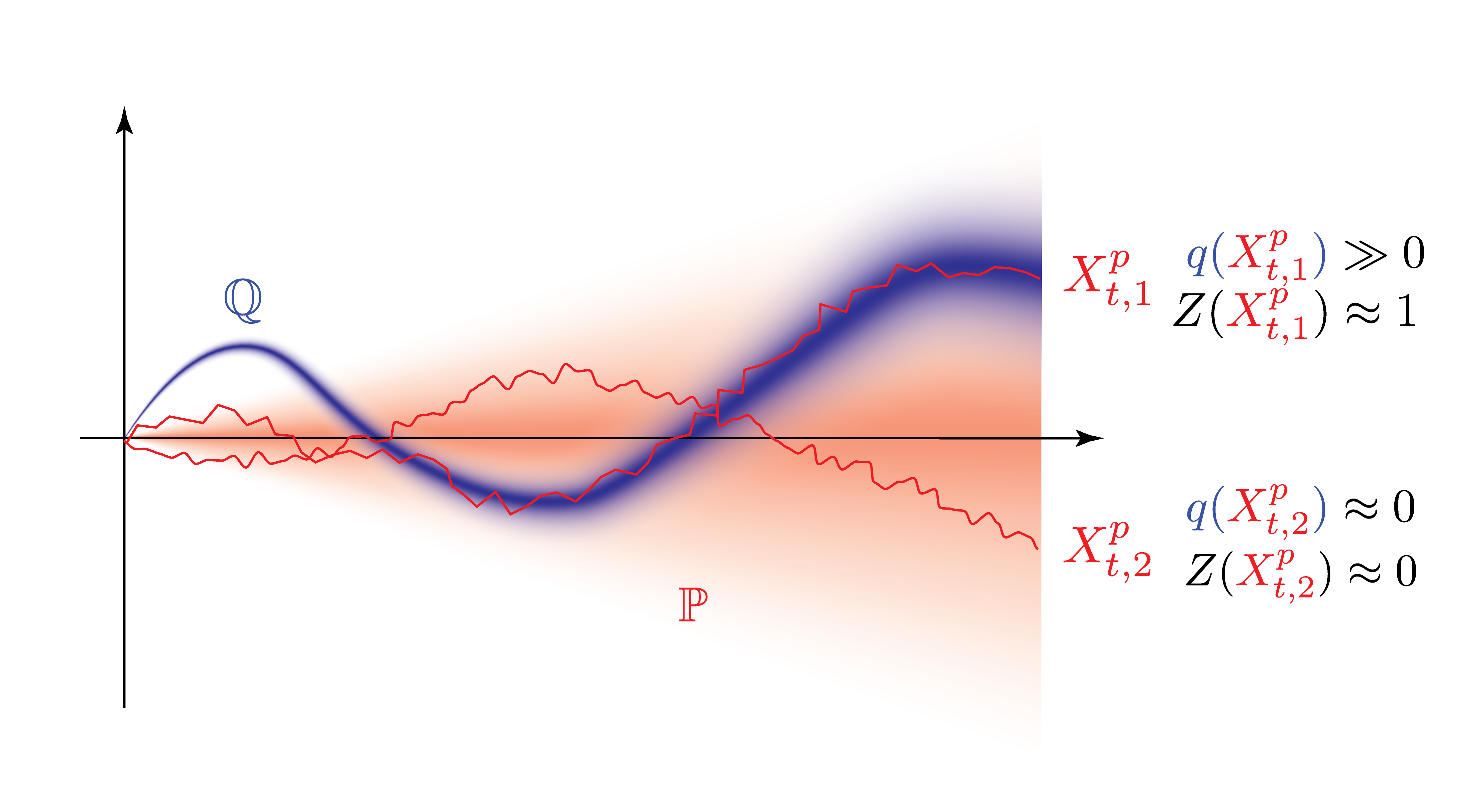
In the draw a series of conclusions from the plot above:

• We sample two realizations of the stochastic process $X^p_{t,1}$ and $X^p_{t,2}$.
• Visually, we can see that whereas $X^p_{t,1}$ ‘hit’ the target measure $\mathbb{Q}$ quite well, $X^p_{t,2}$ did almost not all all.
• Correspondingly, the probability $q(X^p_{t,1})$ is quite high, which makes reweighting $Z(X^p_{t,1})$ close to one, and contributes to the expected value $\mathbb{E}[Z(X^p_{t,1}) f(X^p_t)]$ almost unadulterated.
• The contribution of $X^p_{t,2}$ to the expected value on the other hand has to be downscaled/graded significantely.