Matching Flows and Scores

“Creating noise from data is easy, creating data from noise is generative modelling.”

That was the first sentence in the seminal ‘Score-Based Generative Modelling Through Stochastic Differential Equations’ by Yang Song et al. It introduced a rigorous mathematical framework for A) turning data into noise with a predetermined stochastic process and B) training a neural network to revert this process. While congruent work had been done by other groups and researchers that paper was the starting point that kicked off generative modelling for me by introducing ‘Diffusion Models’.

Diffusion models have delivered a breakthrough in generative modelling thanks to (IMHO) two main properties: simulation-free training and separating the modelling problem into many separate smaller problems. They use a forward process which transforms data into noise over time. During training, we can jump to any time step of this forward process and train the model to make the noisy data slightly less noisy. Just as we can turn data into noise by repeatedly adding just a sliver of noise to it, we can equally denoise data (with the right model) repeatedly to recover the original data.

The data samples are transformed into noise samples by a stochastic process which is defined by a stochastic differential equation (SDE),

We can take a sample $x_0 \sim p(x)$ from the data distribution $p(x)$ and if we simulate the SDE long enough, we will end up with a sample $x_1$ that is indistinguishable (in a statistical sense) from a sample $\epsilon \sim p(\epsilon)$ from the noise distribution $p(\epsilon)$.

The reverse process, which transforms noise samples $\epsilon$ into sample from the data distribution $p(x)$, is defined by the reverse SDE,

where the score function $\nabla_x \log p_\tau(x_\tau)$ is learned by a neural network and the $\alpha$ serves as a hyperparameter.

The free choice of $\alpha$ can revert the original stochastic process in a number of different ways. The formulation of the reverse SDE automatically takes care of the different behaviors of $\alpha$. The score term acts as an optimal control term with which we control the reverse process. If we scale up the diffusion with a large $\alpha$, in turn we automatically act with greater control on the stochastic system. We could also set $\alpha=0$ in which case the Wiener process vanishes and we’re dealing with a deterministic ODE

One interpretation of diffusion model is that we want to connect a data distribution with a noise distribution. Upon successfull training, we can then sample from the noise distribution and transform it into data. The stochastic process at the heart of diffusion models provides this (stochastic) connection.

While we originally started out with the idea of connecting data and noise with a stochastic process, setting $\alpha=0$ in the reverse SDE gives us a deterministic connection.

But does the connection really have to be stochastic at all? The probability flow interpretation of diffusion models suggests that we can also connect data and noise deterministically by setting $\alpha=0$ in the reverse SDE.

Flow Matching Vector Fields

The authors of the original Flow Matching paper followed this chain of thought and directly parameterized the ‘connection’ between the data and the noise distribution with a deterministic vector field. But instead of going through the trouble of deriving a stochastic process that would transform data into noise, they started out from a deterministic map by defining a vector field $v(x_t, t)$ that would transform data samples $x_0$ into noise samples $\epsilon$.

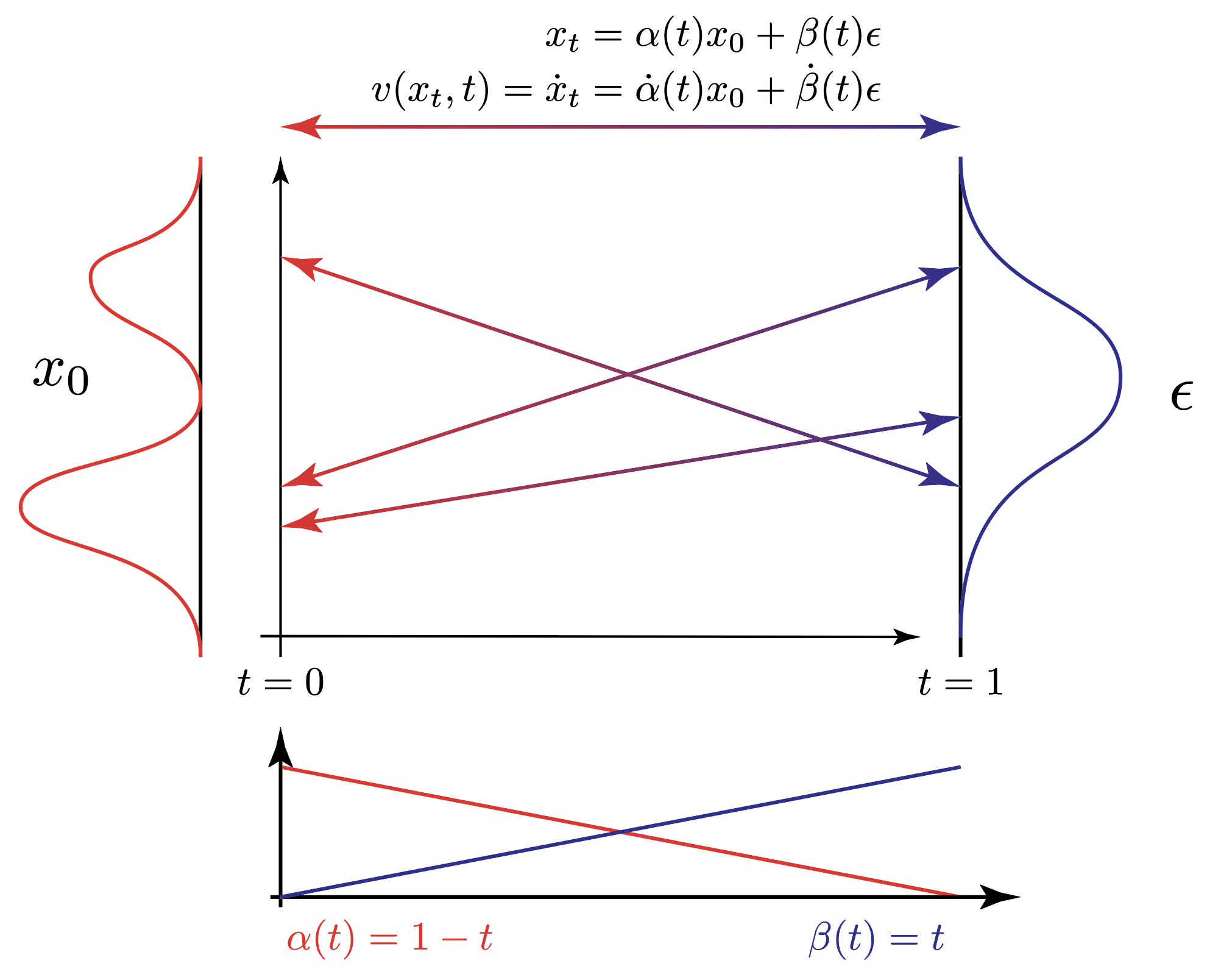
Comparing this with the SDE formulation above, we can see that the vector field $v(x_t, t)$ directly defines a deterministic transformation from data $x_0$ to noise $\epsilon$:

The two terms $\dot{\alpha}(t)$ and $\dot{\beta}(t)$ are the time derivative of the interpolation

where the interpolation functions $\alpha(t)$ and $\beta(t)$ are chosen such that $\alpha(t)$ monotonically decreases from 1 to 0 and $\beta(t)$ monotonically increases from 0 to 1. In fact, they can be chosen as simple as a linear function of time:

And that’s it: we have defined the mathematics of a generative model in less than four straightforward lines of equations. We can take a sample $x$ from the data distribution and transform it into a sample $\epsilon$ from the noise distribution by integrating the vector field $v(x_t, t)$ over time,

The integration above is straightforward and unsurprisingly the equation holds. But also that is the direction that we can model easily since we’re already given a data sample $x_0$. Sampling $\epsilon$ from the noise distribution and computing the interpolation is trivial in this setup.

The reverse direction is more interesting. We want to sample $\epsilon$ and integrate the interpolation backwards such that we obtain a sample from $p(x)$.

For that we parameterize a vector field $v_\theta(x_t, t)$ that transforms noise samples $\epsilon$ into data samples $x_0$. To train we minimize the difference between the vector field $v_\theta(x_t, t)$ and the true vector field $v(x_t, t)$.

This objective function tasks the neural network parameterizing $v_\theta(x_t, t)$ to predict the direct line between $x_0$ and $\epsilon$. Whereas the interpolations are by design crossing each other, the neural network can only settle on a single direction for a $(x_t, t)$ input pair. That’s the reason why we’ll obtain a smooth vector field after training:

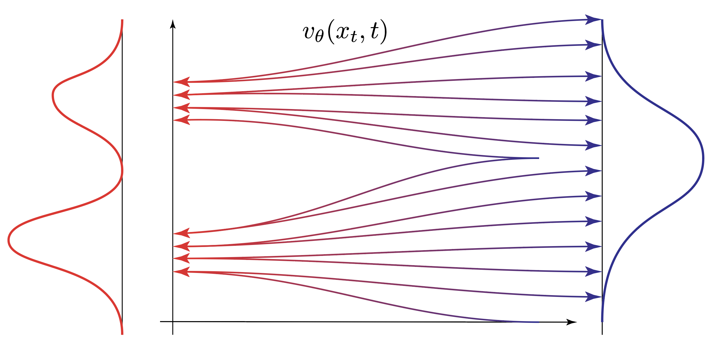
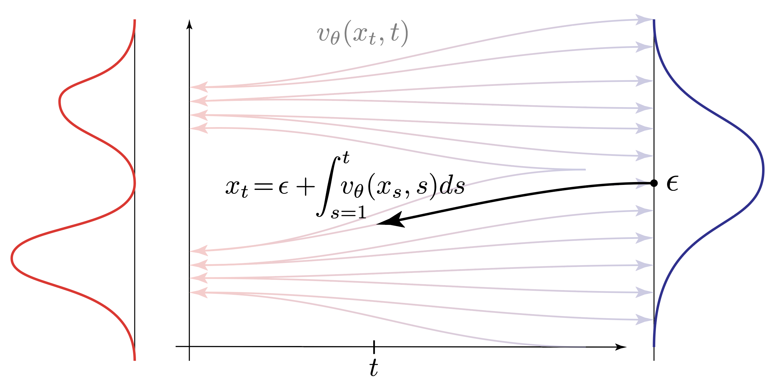
To achieve sampling ‘all’ we have to do is integrate the learned vector field $v_\theta(x_t, t)$ backwards in time from the noise distribution to obtain a sample $x_0$ from the data distribution. In this setup, we don’t have $x_0$ and we will integrate the learned vector field $v_\theta(x_t, t)$ backwards in time to obtain a sample $x_0$ from the data distribution,

Voila, we have a generative model that can sample from the data distribution by integrating a vector field backwards in time.

The Score in Flow Matching

So far we have only talked about the vector field $v(x_t, t)$ and its learned counterpart $v_\theta(x_t, t)$. We saw that the vector field $v(x_t, t)$ directly connects data samples $x_0$ with noise samples $\epsilon$ with a deterministic map. The vector field $v_\theta(x_t, t)$ is trained to approximate this connection. For sampling we have to solve the ODE $dx_\tau = v_\theta(x_\tau, \tau) d\tau$ backwards in time from the noise distribution.

Can we construct an SDE from this vector field, to obtain a stochastic process that connects data and noise? If we can answer this question to the affirmative we would like to have a reverse time SDE in the following form:

So the role of the diffusion term $\sigma(\tau)$ is to introduce noise into the system which we control with the score term $\nabla_x \log p_\tau(x_\tau)$. Remember that setting the diffusion parameter $\sigma(\tau)=0$ would recover our ODE. Adding a Wiener process $dW_\tau$ to the ODE is easy but deriving the correct stochastic control term $\nabla_x \log p_\tau(x_\tau)$ is a whole other story.

In order to derive the score term $\nabla_x \log p_\tau(x_\tau)$ we have to do a quick excursion into the realm of characteristic functions.

Characteristic Functions

What we’re aiming for is to determine the score term $\nabla_x \log p_\tau(x_t)$ from the stochastic process that connects the two random variables $x_0$ and $\epsilon$. But the random variable $x_t$ during sampling is the sum of two random variables $x_0$ and $\epsilon$, namely via $x_t = \alpha(t) x_0 + \beta(t) \epsilon$. The probability distribution of the sum of two random variables is the convolution of the respective probability density functions.

To ease into the topic, we will for starters only consider $Z = X + Y$, where the PDF of $Z$ is consequentially the convolution of the PDFs of $X$ and $Y$:

That doesn’t seem to be the most equation to be working with.

Also, why is actually the convolution of the two PDF’s?

In the case of the sum of $X$ and $Y$ we have to consider all possible values of $X$ and $Y$ that sum up to $Z$. For example, let’s consider the probability of obtaining $Z=5$. We can then first choose $X$ and choose $Y$ as the remainder such that $Y = Z-X$. In order to get $Z=5$ we need to consider the joint probability of all permissible combinations of $X$ and $Y$, so for example $X=2$ and $Y=3$, or $X=3$ and $Y=2$, or $X=4$ and $Y=1$ or $X=-1000$ and $Y=995$. In terms of a decision tree, the convolution symbolizes first choosing $X$ and then choosing $Y = Z - X$ such that ultimately $X+Y=Z$.

Computing the convolution would be a bit of a hassle. But fortunately, we can use the Fourier transform to turn this into a more amenable expression. People with signal processing experience will already know that the convolution in the spatial domain corresponds to the multiplication in the frequency domain. Thus if we can apply the Fourier transform to the two respective PDF’s $p(x)$ and $p(y)$, we can instead just multiply them and then transform the resulting PDF back to the spatial domain,

where $\hat{p} = \text{FT}\left[ p \right]$ is the Fourier transform of a function $p$ and $\text{IFT}$ is the inverse Fourier transform. Remember that probability density functions are also just functions with some particular properties.

But how do we apply the Fourier transform to a random variable? We interpret the probability density function $p(x)$ just like a regular function and on the way we absorb $-2\pi$ into $k$ to obtain the characteristic function of the random variable $X$.

Applying the Fourier transformation on a PDF gives us, what is referred to as, the characteristic function of the random variable.

We can easily apply the Fourier transform to the sum of two random variables $Z = X + Y$, and obtain

Next we apply a change of variable $y = z - x$ from which follows that $z = x + y$ and by differentiation $dz = dy$,

It should be noted that the separation of the two random variables $X$ and $Y$ in the Fourier domain is a direct consequence of their independence. But this bodes well for our original problem of the sum of two random variables $x_t = \alpha(t) x_0 + \beta(t) \epsilon$ where the random variables $x_0$ and $\epsilon$ are chosen to be statistically independent by design.

As it will become important for the derivation of the score term, we will now consider the characteristic function of a multivariate Normal distribution,

One of the big advantages of the characteristic function is that it is easy to compute moments of the corresponding distribution by simply deriving once for the first moment and twice for the second moment and setting $k=0$ and multiplying the result by $i^{-k}$ where $k$ denotes the order of the moment. For the Gaussian example above, all we have to do is

which is the rearranged definition of the variance $\Sigma = \mathbb{E}[x^2] - \mathbb{E}[x]^2$.

For a scaled but centered Gaussian distribution $\mathcal{N}(0, \sigma^2 \text{I})$ we have the characteristic function

which will be of importance for defining the score term in the flow matching approach

The (Fundamental) Score Term

In the following, we will try (and suceed) to express the conditional noise $\mathbb{E}[\epsilon | x_t]$ with characteristic functions.

Let’s consider the equation

where we used the law of iterated expectations.

The left hand side can be rewritten as

Combining the two expressions we obtain

Where we used the nice property of integration by parts on probability density functions which evaluate to $0$ at the boundaries of $x=\pm \infty$. If we consider a test function $f(x)$ and a probability density function $p(x)$, we have

Putting these two expressions together we obtain it will only hold if the differing terms actually equate to each other, namely

Obtaining Scores from the Vector Field

plot that with x and vector field allows estimating epsilon and data, ‘projection’

Flow matching trains a neural network to approximate the vector field $v(x_t, t)$. Given a data sample $x_t$ we can then extract the conditional expectation of both $x_0$ and $\epsilon$ from the vector field $v(x_t, t)$. Intuitively, this can be achieved by projecting via the vector field $v(x_t, t)$ from the data sample $x_t$ to the noise sample $\epsilon$ and back to the data sample $x_0$. Remember that this is how we defined the vector field $v(x_t, t)$ in the first place.

We can actually gain some insight into the score term by reducing the score estimator and plugging in the linear interpolation functions $\alpha(t) = 1-t$ and $\beta(t) = t$ and $\dot{\alpha}(t) = -1$ and $\dot{\beta}(t) = 1$.

Here, $\epsilon$ is the best guess we can estimate given the data sample $x_t$ and the vector field $v_\theta(x_t, t)$. Looking at the drift of the reverse time SDE, we can simplify things to

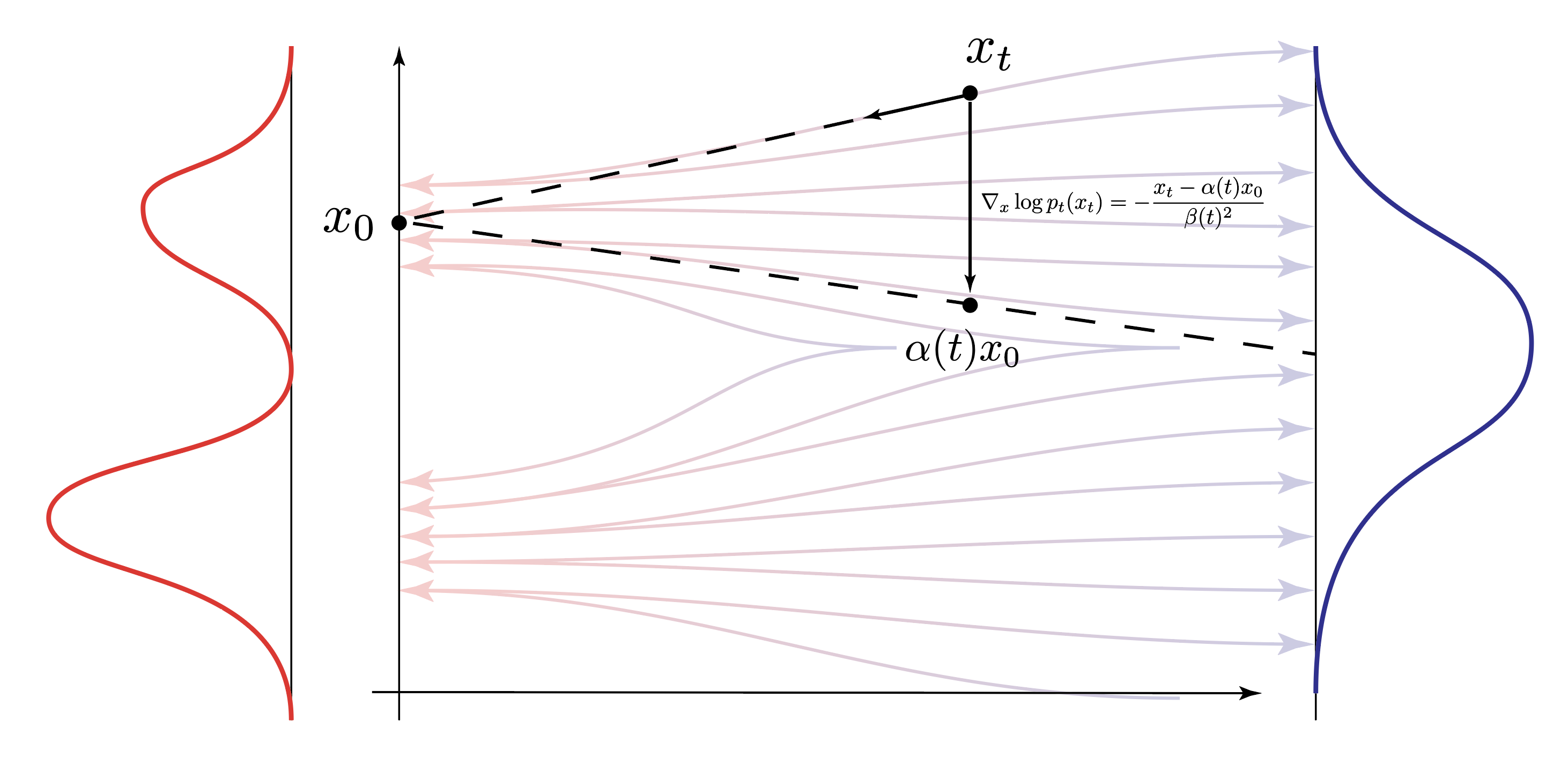
The score in the flow matching approach pushes the sample $x_t$ towards what it believes is the interpolated data $\alpha(t) x_0$. Close to the noise, this will naturally be very close around $0$, as the noise is centered around $0$. But as we’re approaching the data sample $x_0$, the score term will push the sample $x_t$ towards the data sample $x_0$.

We can in fact compare this to the score of a in a DDPM model with attenuation $\alpha(t)$ and noise $\sigma(t)$. The forward process can be sampled in an almost identical fashion to the flow matching model. DDPM models differ in their choice of $\alpha(t)$ and $\sigma(t)$ which are analogous in the continuous time limit to the Ornstein Uhlenbeck process.

Sampling $x_t$ in a DDPM model is functionally identical to the flow matching model.

Since DDPM is built on the Ornstein Uhlenbeck process, the score term is given by by the gradient of the log marginal probability density function of a time-dependent Gaussian:

where all the relevant terms occur in a similar fashion to the flow matching model.

Let’s try it out with some Code

So let’s try this out with some code. One thing to note, and what I personally think is nice, is that the interpolation paramters $\alpha(t)$, $\beta(t)$ can be chosen independently from the diffusion parameter $\sigma(t)$.

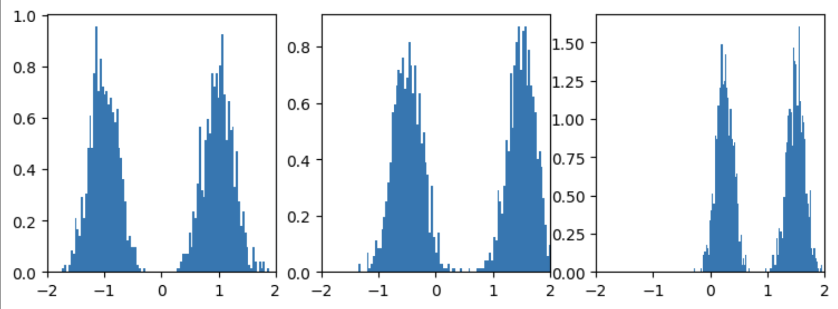
Let’s generate some data in form of a 3D GMM:

import torch
import einops
import matplotlib.pyplot as plt

'''Generate Samples from a rudimentary GMM'''
means = torch.Tensor([[-1, 1], [-0.5, 1.5], [1.5, 0.25]])
stds = torch.Tensor([[0.25], [0.25], [0.15]]).repeat((1,2))
means.shape, stds.shape
num_samples = 1_000
gmm = torch.distributions.Normal(loc=means, scale=stds)
samples = einops.rearrange(gmm.sample((num_samples,)), 'n d c -> (n c) d')
samples.shape

'''Visualize GMM Samples'''
fig, axs = plt.subplots(1,3, figsize=(9,3))
for dim in range(samples.shape[1]):
    axs[dim].hist(samples[:,dim], density=True, bins=100)
    axs[dim].set_xlim(-2,2)
plt.show()

Let’s define the flow matching model and the loss function:

from torch.nn import Sequential, Module, Linear, ELU, GELU
import tqdm
class FlowMatchingModule(Module):
    def __init__(self, dim=2, pos_emb_dim=2, hidden=64, net=None):
        super().__init__()
        self.dim = dim
        self.pos_emb_dim = pos_emb_dim
        if not net:
            self.net = Sequential(
                Linear(dim + pos_emb_dim, hidden), # R^Input x R_[0,1] -> R^Hidden
                GELU(),
                Linear(hidden, hidden), GELU(),
                Linear(hidden, hidden), GELU(),
                Linear(hidden, hidden), GELU(),
                Linear(hidden, dim))
        else:
            self.net = net
        self.t_emb = Linear(1, pos_emb_dim//2)

    def forward(self, t, x):
        t = self.t_emb(t).mul(torch.pi)
        t = torch.cat((t.cos(), t.sin()), dim=-1)
        return self.net(torch.cat((t, x), dim=-1))

def ot_loss(model, x):
        '''Learns the vector field from data to noise'''
        time = torch.rand(len(x), 1).to(x.device) # random time t ~ U(0,1)
        noise = torch.randn_like(x) # noise distribution epsilon ~ N(0,1)
        noisedx = (1 - time) * x + (0.001 + 0.999 * time) * noise # OT interpolation with time stabilization
        target = noise.mul(0.999) - x # vector from data to noise
        prediction = model(time, noisedx)
        return (prediction - target).square() # compute per dim per sample loss

Let’s write the Runge-Kutta 4 integrator and the sampling function:

@torch.no_grad()
def sample(model, num_samples, num_steps=20, show_traj=False):
    device = next(model.parameters()).device
    x = torch.randn((num_samples, model.dim)).to(device)
    dt = 1.0 / num_steps
    traj_data_prediction = []
    for i, t in tqdm.tqdm(enumerate(torch.linspace(1, 0, num_steps))):
        t = t.expand(len(x), 1).to(device)
        if True: # RK4
            k1 = model(t, x)
            k2 = model(t - dt/2, x - (dt*k1)/2)
            k3 = model(t - dt/2, x - (dt*k2)/2)
            k4 = model(t - dt, x - dt*k3)
            dx = (k1 + 2*k2 + 2*k3 + k4) / 6
            x = x - dt *dx
            if i%(num_steps//10)==0:
                traj_data_prediction += [x - t*dx]
        else:
            x = x - dt * (model(t,x))

    if show_traj:
        fig, axs = plt.subplots(1, len(traj_data_prediction), figsize=(30,3))
        for i, data in enumerate(traj_data_prediction):
            axs[i].hist(data[:,0].cpu().numpy(), density=True, bins=100)
            axs[i].set_ylim(0,1)
            axs[i].set_xlim(-2,2)
            axs[i].set_title(f'Integration Time t={1-i/len(traj_data_prediction):.2f}')
        fig.suptitle('Predicted target tilde{x} of generative Process (Direction: noise -> data)')
        plt.tight_layout()
        plt.show()

    return x

and visualize the samples and the intermediate trajectories

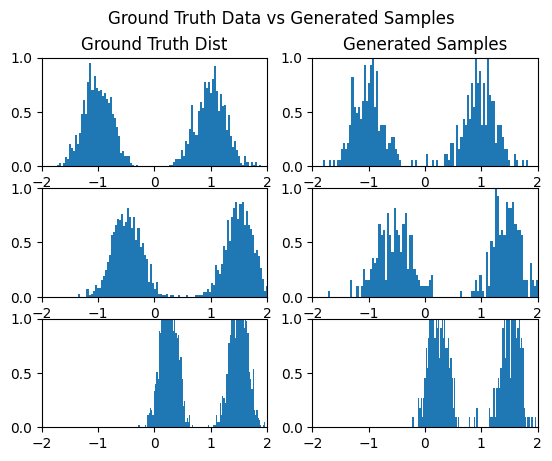
gen_samples = sample(model, 500, num_steps=1000, show_traj=True).cpu().numpy()
print(gen_samples.shape)

fig, axs = plt.subplots(3,2)
for dim in range(samples.shape[1]):
    axs[dim,1].hist(gen_samples[:,dim], density=True, bins=100)
    axs[dim,0].hist(samples[:,dim], density=True, bins=100)
    axs[dim,0].set_xlim(-2,2)
    axs[dim,0].set_ylim(0,1)
    axs[dim,1].set_xlim(-2,2)
    axs[dim,1].set_ylim(0,1)

axs[0,0].set_title('Ground Truth Dist')
axs[0,1].set_title('Generated Samples')
fig.suptitle('Ground Truth Data vs Generated Samples')
plt.show()

Now let’s do some SDE sampling

def sample_sde(model, n_samples, num_steps=100, show_traj=False):
        """
        x_t = (1 - t) * x + t * noise
            = α * x + σ * noise
        score(velocity):
            s(x,t) = σ_t^-1 ( α v(x,t) - dα/dt x ) / (dα/dt * σ_t - α_t * dσ_t/dt )^2
        """
        x = torch.randn((n_samples, 3)).to(device)
        dt = 1.0 / num_steps

        alpha_t = lambda t: 1 - t
        dalpha_t = -1
        sigma_t = lambda t: 0.001 + 0.999 * t
        dsigma_t = 0.999
        traj_data_prediction = []
        with torch.no_grad():  # runge-kutta-4 diffeq solver
            for i, t in tqdm.tqdm(enumerate(torch.linspace(1, 0, num_steps))):
                t = t.expand(len(x), 1).to(device)
                v = model(t, x)
                score = (
                    1
                    / (sigma_t(t) + 1e-6)
                    * (alpha_t(t) * v - dalpha_t * x)
                    / (dalpha_t * sigma_t(t) - alpha_t(t) * dsigma_t + 1e-6)
                )
                dx = v * dt
                dx += -1 / 2 * sigma_t(t) * score * dt
                dx += (sigma_t(t) * dt).pow(0.5) * torch.randn_like(x)
                x = x - dx
                if i%(num_steps//10)==0:
                    traj_data_prediction += [x - t*dx]
        if show_traj:
            fig, axs = plt.subplots(1, len(traj_data_prediction), figsize=(30,3))
            for i, data in enumerate(traj_data_prediction):
                axs[i].hist(data[:,0].cpu().numpy(), density=True, bins=100)
                axs[i].set_ylim(0,1)
                axs[i].set_xlim(-2,2)
                axs[i].set_title(f'Integration Time t={1-i/len(traj_data_prediction):.2f}')
            fig.suptitle('Predicted target tilde{x} of generative Process (Direction: noise -> data)')
            plt.tight_layout()
            plt.show()
        return x

And visualize the SDE samples:

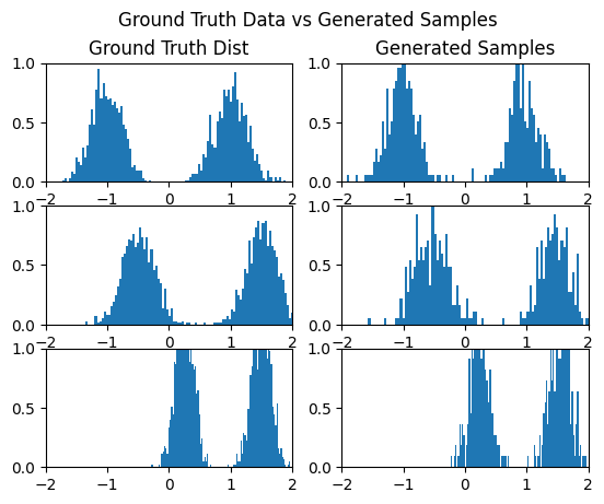
gen_samples = sample_sde(model, 500, num_steps=1000, show_traj=True).cpu().numpy()
print(gen_samples.shape)

fig, axs = plt.subplots(3,2)
for dim in range(samples.shape[1]):
    axs[dim,1].hist(gen_samples[:,dim], density=True, bins=100)
    axs[dim,0].hist(samples[:,dim], density=True, bins=100)
    axs[dim,0].set_xlim(-2,2)
    axs[dim,0].set_ylim(0,1)
    axs[dim,1].set_xlim(-2,2)
    axs[dim,1].set_ylim(0,1)

axs[0,0].set_title('Ground Truth Dist')
axs[0,1].set_title('Generated Samples')
fig.suptitle('Ground Truth Data vs Generated Samples')
plt.show()

What I find interesting is that the ODE samples settle quite quickly on the bifurcation of the GMM: Already at 40% of the integration time, the samples are quite close to the GMM.

Compare that to the SDE sample which takes a bit longer to settle on the GMM: Only in the last 30% or so are the modes actually captured. This is actually very close to classic diffusion models where the schedules are chosen in such a way that a perceptual sample only crystallizes close to the end of the sampling process.

Coolio, that’s it for today.