12 Jul 2025

Feynman-Kac

Is it Katz, Kak, Kaz, Katsch? Anyway, it's nice math.

Recently there has been quite interest in the idea of Feynman-Kac Steering.

For a given diffusion model, we can generate samples by iteratively removing noise, transforming a sample of pure noise into a sample of the target distribution. At each step during the denoising process we can let the model estimate what the fully denoised sample would look like. This can happen either through the score identity or is even more readily available if the model was trained on a denoising loss. These fully denoised samples are then evaluated with a criterion. This criterion is then “pulled back” into the denoising process to gauge whether the sample is going to be sufficiently good if fully denoised. Feynman-Kac steering the implements a resampling step where all the samples are evaluated with the criterion in parallel and the batch is resampled from the noisy samples proportional to each samples fully denoised criterion. This is essentially particle filtering with extra steps with stochastic PDE theory wrapped around it.

So let’s dissect the theory.

Ito Derivative

At the core of diffusion model is a stochastic process $X_t$ that evolves according to a stochastic differential equation (SDE). The Ito derivative is a key concept in stochastic calculus that allows us to differentiate functions of stochastic processes.

The SDE in question is typically of the form: $dX_t = \mu(X_t, t) dt + \sigma(X_t, t) dW_t$ where $\mu$ is the drift term, $\sigma$ is the diffusion term, and $W_t$ is a Wiener process (or Brownian motion).

What happens to a function $f(X_t, t)$ as it evolves over time? The Ito derivative gives us a way to compute this by extending the classical Taylor expansion to the stochastic process realm:

$$ \begin{align*} f(X_{t+\Delta t}, t+ \Delta t) =& f(X_t, t) + \frac{\partial f(X_t, t)}{\partial t} (t + \Delta t - t) + \frac{\partial f(X_t, t)}{\partial X_t} (X_{t+\Delta t} - X_t) \\ &+ \frac{1}{2} \frac{\partial^2 f(X_t, t)}{\partial X_t^2} (X_{t+\Delta t} - X_t)^2 + o(\Delta t) \end{align*} $$

An important factor that we’ll encounter in a second again is that we won’t consider effects of higher order as A) they get divided by ever decreasing factors and B) they are negligible for small $\Delta t^p$ where $p>2$.

We then get the Ito derivative:

$$ \begin{align*} f(X_{t+\Delta t}, t+ \Delta t) =& f(X_t, t) + \frac{\partial f(X_t, t)}{\partial t} \Delta t + \frac{\partial f(X_t, t)}{\partial X_t} (X_{t+\Delta t} - X_t) \\ &+ \frac{1}{2} \frac{\partial^2 f(X_t, t)}{\partial X_t^2}(X_{t+\Delta t} - X_t)^2 + \cancel{o(\Delta t)} \\ % &= f(X_t, t) + \frac{\partial f(X_t, t)}{\partial t} \Delta t + \frac{\partial f(X_t, t)}{\partial X_t} (X_{t+\Delta t} - X_t) \\ % &+ \frac{1}{2} \frac{\partial^2 f(X_t, t)}{\partial X_t^2} (X_{t+\Delta t} - X_t)^2 \end{align*} $$

For an infinitesimally small time increment $\Delta t$, we assume that the difference becomes a continuous $dt$ and we can plug in our SDE:

$$\begin{align*} f(X_{t+\Delta t}, t+ \Delta t) =& f(X_t, t) + \frac{\partial f(X_t, t)}{\partial t} dt + \frac{\partial f(X_t, t)}{\partial X_t} \overbrace{(X_{t+\Delta t} - X_t)}^{=dX_t} \\ &+ \frac{1}{2} \frac{\partial^2 f(X_t, t)}{\partial X_t^2} \overbrace{(X_{t+\Delta t} - X_t)^2}^{=dX_t^2} \\ =& f(X_t, t) + \frac{\partial f(X_t, t)}{\partial t} dt + \frac{\partial f(X_t, t)}{\partial X_t} (\mu(X_t, t)dt + \sigma(X_t, t) dW_t) \\ &+ \frac{1}{2} \frac{\partial^2 f(X_t, t)}{\partial X_t^2} (\mu(X_t, t)dt + \sigma(X_t, t) dW_t)^2 \\ =& f(X_t, t) + \frac{\partial f(X_t, t)}{\partial t} dt + \frac{\partial f(X_t, t)}{\partial X_t} (\mu(X_t, t)dt + \sigma(X_t, t) dW_t) \\ &+ \frac{1}{2} \frac{\partial^2 f(X_t, t)}{\partial X_t^2} (\mu(X_t, t)^2dt^2 + 2\mu(X_t, t)\sigma(x_t, t) dt dW_t + \sigma(X_t, t)^2 dW_t^2) \\ \end{align*}$$

The next step to observe is that $dW_t = \epsilon \sqrt{dt}$ and that in the limit for a very small $dt$ (think of $dt=10^{-5}$), any effect of a term with $dt$ raised to any power larger than $1$ will diminish even faster (think of $dt^{1.5}=(10^{-5})^{1.5} = 10^{-7.5}$) and thus become negligible. This allows us to drop any term where $dt^p$ where $p>1$. Isn’t math convenient?

We thus get

$$\begin{align*} f(X_{t+\Delta t}, t+ \Delta t) =& f(X_t, t) + \frac{\partial f(X_t, t)}{\partial t} dt + \frac{\partial f(X_t, t)}{\partial X_t} (\mu(X_t, t)dt + \sigma(X_t, t) dW_t) \\ &+ \frac{1}{2} \frac{\partial^2 f(X_t, t)}{\partial X_t^2} (\underbrace{\cancel{\mu(X_t, t)^2dt^2}}_{dt^2 \rightarrow 0} + \underbrace{\cancel{2\mu(X_t, t)\sigma(x_t, t) dt dW_t}}_{dt^{1.5} \rightarrow 0} + \sigma(X_t, t)^2 \underbrace{dW_t^2}_{=dt}) \\ =& f(X_t, t) + \frac{\partial f(X_t, t)}{\partial t} \Delta t + \frac{\partial f(X_t, t)}{\partial X_t} (\mu(X_t, t)dt + \sigma(X_t, t) dW_t) \\ &+ \frac{1}{2} \frac{\partial^2 f(X_t, t)}{\partial X_t^2}\sigma(X_t, t)^2 dt \end{align*}$$

Rearranging a bit we have

$$\begin{align*} f(X_{t+\Delta t}, t+ \Delta t)- f(X_t, t) =& \frac{\partial f(X_t, t)}{\partial t} dt + \frac{\partial f(X_t, t)}{\partial X_t} (\mu(X_t, t)dt + \sigma(X_t, t) dW_t) \\ &+ \frac{1}{2} \frac{\partial^2 f(X_t, t)}{\partial X_t^2}\sigma(X_t, t)^2 dt \end{align*} $$

So the infinitesimal change on the right hand side, properly denoted by $dt$ and $dW_t$, would equate the difference in the function $f(X_{t+\Delta t}, t+ \Delta t)$ and $f(X_t, t)$. Given a step of $dt$ in time, the change in the function $f(X_t, t)$ is given by

$$ \begin{align*} df(X_t, t) =&\left\{\frac{\partial f(X_t, t)}{\partial t} + \frac{\partial f(X_t, t)}{\partial X_t} \mu(X_t, t) + \frac{1}{2} \frac{\partial^2 f(X_t, t)}{\partial X_t^2}\sigma(X_t, t)^2\right\} dt \\ & + \sigma(X_t, t) \frac{\partial f(X_t, t)}{\partial X_t} dW_t \end{align*}$$

Backward Kolmogorov Equation

Ito’s lemma gives us a way to compute the infinitesimal change in a function of a stochastic process. Since our process is stochastic, for any realized $x_t$, if we run the stochastic process again, we will get a different $X_T$ where $T= t + \Delta t$. All the stochasticity that we accrue over time $\Delta t$ will make the function $f(X_T, T)$ a random variable.

As a sort of cognitive crutch, you can think of $f(X_T)$ as your Temple Run gold coin counter. You always start from the same starting point $x_t$ and you always do the same 5 moves in the time $\Delta t$. If the coin positions stay fixed and you do the same five moves every time you run, you’ll always get the same score $f(x_T)$ at the end. This is what the deterministic part models. But now the stochastic parts keeps on changing the gold coin positions. Even for a fixed score $f(x_t)$ and deterministic moves/dynamics, you final gold coin score $f(x_T)$ will vary. Sometimes you’ll get a lot of gold coins, sometimes you’ll get none. So essentially, you’re gold coin score $f(X_T)$ now is a random variable.

The next question we have to ask to naturally arrive at the Kolmogorov backward equation is whether there is a function $f_T(x_T)$ that describes the expected value of $f_T(X_T)$ for the current state $x_t$ given that the dynamics are stochastic!

So we’d be interested in the equation

$$ \begin{align*} f(x_t, t) &= \mathbb{E} \left[ f_T(X_T) | X_t = x_t \right] \\ &= \int \underbrace{p(X_T = x_T|x_t)}_{\text{Stochastic Process}} f_T(X_T) dx_T \end{align*} $$

where the expectation how likely a state $X_T$ is given the current state $x_t$ is given by the stochastic process $p(X_T | x_t)$. So $f_T(x_T)$ gives you an estimate of how much payout at the end you’ll get midway through your Temple Run.

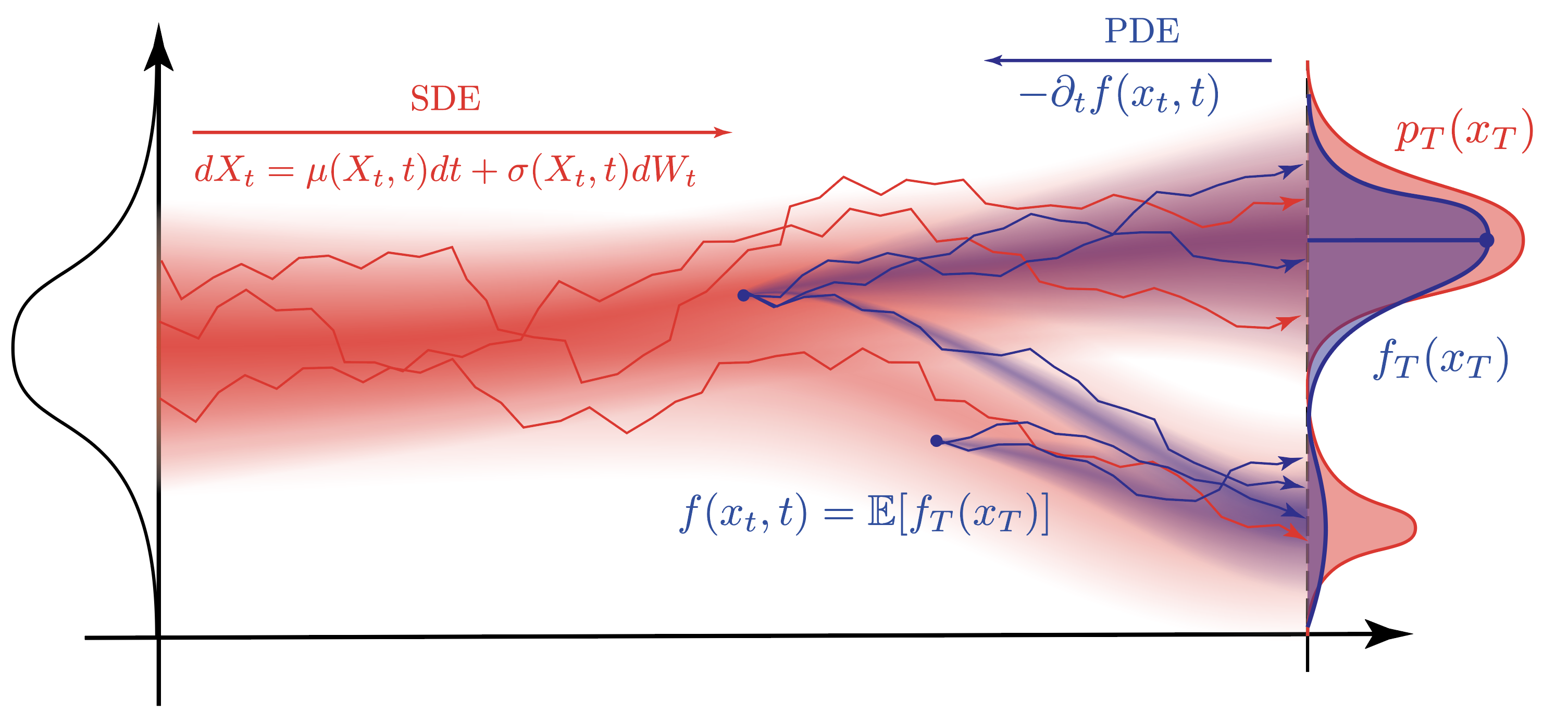
Figure: Visual intuition for Feynman-Kac. The stochastic process $X_t$ evolves under random noise, while the expected value of a terminal criterion $f_T(X_T)$ is “pulled back” to earlier times via the backward PDE. Particle trajectories (red) and expectation (blue) illustrate the connection between stochastic paths and deterministic backward evolution.

But the definition $f_T(x_T)$ is inherently forward looking as it relies on the solving the SDE forward in time. Can we also reverse time in a way to compute earlier values of $f(x_t,t)$ starting from the terminal values $f_T(X_T)$?

It turns out that there is a partial differential equation hidden beneath all this stochasticity that allows us to compute the expected value of $f(x_t, t)$ backwards in time.

To show this we’ll start out with Ito’s lemma above but this time integrate it all the way from $t$ to $T$.

$$ \begin{align*} f_T(X_T) | X_t =& f(X_t, t) + \int_t^T \left\{\frac{\partial f(X_t, t)}{\partial t} + \frac{\partial f(X_t, t)}{\partial X_t} \mu(X_t, t) + \frac{1}{2} \frac{\partial^2 f(X_t, t)}{\partial X_t^2}\sigma(X_t, t)^2\right\} dt \\ & + \int_t^T \sigma(X_t, t) \frac{\partial f(X_t, t)}{\partial X_t} dW_t \end{align*} $$

(where I should have used the integration variable $s$ or $\tau$ instead of $t$ but I didn’t want to introduce unnecessary notational noise ;-) ). More importantly, this equation tells us that if we start with some intermediate value $f(X_t, t)$ and integrate the infinitesimal changes in the function $f(X_t, t)$ from $t$ to $T$, we will end up with the final value of the function $f_T(X_T)$ which is our terminal payout.

And now comes the important step …

… drumroll 🥁 …

… we take the expectation. 👍

The important thing to note is that the expectation of a Wiener process, however he might be scaled over any time, is zero.

$$ \begin{align*} \mathbb{E}\left[ f_T(X_T) | X_t \right] =& \mathbb{E} \left[ f(X_t, t) + \int_t^T\left\{\frac{\partial f(X_t, t)}{\partial t} + \frac{\partial f(X_t, t)}{\partial X_t} \mu(X_t, t) + \frac{1}{2} \frac{\partial^2 f(X_t, t)}{\partial X_t^2}\sigma(X_t, t)^2\right\} dt \right] \\ & + \underbrace{\cancel{\mathbb{E}\left[\sigma(X_t, t) \frac{\partial f(X_t, t)}{\partial X_t} dW_t \right]}}_{=0} \end{align*} $$

While $X_t$ is a random variable, its stochasticity arises completely from the input of the Wiener process $dW_t$. If we eliminate the influence of the Wiener process with the expectation $\mathbb{E}$ at every step, we will essentially obtain a deterministic ODE. With this intuition, the expectation essentially has no influence on the remaining terms and we can write

$$ \begin{align*} \underbrace{\mathbb{E}\left[ f_T(x_T) | X_t \right]}_{=f(X_t, t)} &= f(X_t, t) + \int_t^T\left\{\frac{\partial f(X_t, t)}{\partial t} + \frac{\partial f(X_t, t)}{\partial X_t} \mu(X_t, t) + \frac{1}{2} \frac{\partial^2 f(X_t, t)}{\partial X_t^2}\sigma(X_t, t)^2\right\} dt \\ f(X_t, t) &= f(X_t, t) + \int_t^T\Bigg\{ \underbrace{\frac{\partial f(X_t, t)}{\partial t} + \frac{\partial f(X_t, t)}{\partial X_t} \mu(X_t, t) + \frac{1}{2} \frac{\partial^2 f(X_t, t)}{\partial X_t^2}\sigma(X_t, t)^2}_{\stackrel{!}{=} 0}\Bigg\} dt \end{align*} $$

The equation above can only hold if the term we’re integrating

$$ \begin{align*} 0 &\stackrel{!}{=} \int_t^T \left\{\frac{\partial f(X_t, t)}{\partial t} + \frac{\partial f(X_t, t)}{\partial X_t} \mu(X_t, t) + \frac{1}{2} \frac{\partial^2 f(X_t, t)}{\partial X_t^2}\sigma(X_t, t)^2 \right\} dt \end{align*} $$

An important observation is that the integral above is a definite integral over the arbitrary time interval $[t, T]$. This means that the integrand must be zero for all $t$ in the interval $[t, T]$ as we could choose $t$ arbitrarily close to $T$ and the integral would still have to be zero. We can go backward in time from the terminal time $T$ to $T-dt$ and the integral has to be zero, i.e. $\int_{T-dt}^T \ldots dt = 0$. If that integral is zero, then the integral $\int_{T-2dt}^{T-dt} \ldots dt = 0$ also has to be zero in order for the whole integral $\int_{T-2dt}^T \ldots dt = 0$ to hold. This means that the integrand must be zero for all $t$ in the interval $[t, T]$. This gives us the backward Kolmogorov equation:

$$ \begin{align*} -\frac{\partial f(X_t, t)}{\partial t} &= \frac{\partial f(X_t, t)}{\partial X_t} \mu(X_t, t) + \frac{1}{2} \frac{\partial^2 f(X_t, t)}{\partial X_t^2}\sigma(X_t, t)^2 \end{align*} $$

with some terminal condition $f_T(X_T)$. This result is quite remarkable as it allows us to compute the expected value of a function of a stochastic process at an earlier time $t$ given the terminal condition $f_T(X_T)$ with a PDE backward in time instead of solving a SDE forward in time.

While it looks deceptively similar to the Ito derivative, the backward Kolmogorov equation is a PDE that describes how the expected value of a function of a stochastic process evolves backward in time.

In practical terms, this means that if we have a function $f_T(X_T)$ at the terminal time $T$ with the stochastic dynamics of $dX_t$, we can compute the expected value of this function at an earlier time $t$ by solving the backward Kolmogorov equation.

For example, we could redefine the function $f_T(X_T)$ as the probability of $p(x_T)$ at the terminal time $T$. We could then solve the Kolmogorov backward equation in the form of a PDE backwards in time to obtain the expected value of the probability at an earlier time $t$, which we would denote as $p(X_T | X_t)$.

$$ \begin{align*} - \frac{\partial p(X_T | X_t)}{\partial t} =& \frac{\partial p(X_T|X_t)}{\partial X_t} \mu(X_t, t) + \frac{1}{2} \frac{\partial^2 p(X_T | X_t)}{\partial X_t^2}\sigma(X_t, t)^2 \end{align*} $$

This equation would evolve backward the probability density $p(X_T | X_t)$ from the terminal time $T$ to the earlier time $t$. At some earlier point $t$, we could evaluate the how likely the state $X_T$ would be given the earlier state $X_t$.

A Stochastic Sidenote

For some function $f(x_t, t)$ and a terminal value $f_T(x_T)$, we derived the following identity above

But now with our previously gained knowledge we can ascertain that the deterministic integrand is always zero, so we obtain the following equation

$$ \begin{align*} f_T(X_T) | X_t =& f(X_t, t) + \int_t^T \sigma(X_t, t) \frac{\partial f(X_t, t)}{\partial X_t} dW_t \end{align*} $$

which is A) a martingale and B) a random variable due to the Ito integral. We can make this more precise by observing as before that the expectation is zero because $\mathbb{E}[dW_t] = 0$. Also, we can quite easily compute the variance of this random variable by computing

$$ \begin{align*} \mathbb{E}\left[ \left( \int_t^T \sigma(X_t, t) \frac{\partial f(X_t, t)}{\partial X_t} dW_t \right)^2 \right] &= \mathbb{E}\left[ \left( \int_t^T \sigma(X_t, t) \frac{\partial f(X_t, t)}{\partial X_t} dW_t \right) \left( \int_t^T \sigma(X_{t'}, {t'}) \frac{\partial f(X_{t'}, {t'})}{\partial X_{t'}} dW_{t'} \right) \right]. \end{align*} $$

By definition a Wiener process $W_t$ has the property that $\mathbb{E}[dW_t dW_{t’}] = \delta(t-t’) dt$ which says that the product of a Wiener process at two different times is zero unless the two times are the same. This means that we can rewrite the above equation as

$$ \begin{align*} \mathbb{E}\left[ \left( \int_t^T \sigma(X_t, t) \frac{\partial f(X_t, t)}{\partial X_t} dW_t \right)^2 \right] &= \int_t^ T \int_t^T \mathbb{E}\left[ \sigma(X_t, t) \frac{\partial f(X_t, t)}{\partial X_t} \sigma(X_{t'}, {t'}) \frac{\partial f(X_{t'}, {t'})}{\partial X_{t'}} dW_t dW_{t'} \right] \\ &= \int_t^T \sigma(X_t, t)^2 \frac{\partial f(X_t, t)}{\partial X_t}^2 dt \end{align*} $$

because all the “cross terms” where $t \neq t’$ vanish due to the property of the Wiener process. This is also known as Ito Isometry. This gives us the mean and variance of the random variable $f_T(X_T) | X_t$:

$$\begin{align*} \mathbb{E}[f_T(X_T) | X_t] &= f(X_t, t) \\ \text{Var}[f_T(X_T) | X_t] &= \int_t^T \sigma(X_t, t)^2 \frac{\partial f(X_t, t)}{\partial X_t}^2 dt \\ &\downarrow \\ f_T(X_T) | X_t &\sim \mathcal{N}\left(f(X_t, t), \int_t^T \sigma(X_t, t)^2 \frac{\partial f(X_t, t)}{\partial X_t}^2 dt\right) \end{align*}$$

Feynman-Kac Equation

Previously, we’ve observed how with a terminal condition at time $T$, we can compute the expected value of a function of a stochastic process at an earlier time $t$ by solving the backward Kolmogorov equation

where the dynamics of a stochastic process $X_t$ are given by the SDE $dX_t = \mu(X_t, t) dt + \sigma(X_t, t) dW_t$ and the terminal condition is given by $f_T(X_T)$.

In their famous equation, Mark Kac and Richard Feynman asked “Yo, what if we add more terms to the Kolmogorov Backward Equation?” (essentially … please don’t quote me on this).

In order to align with the normal notation of the Feynman-Kac equation, we will be using $u$ instead of $f$. The FK equation then is posited as follows:

$$ \begin{align*}-\frac{\partial u(X_t, t)}{\partial t} &= \frac{\partial u(X_t, t)}{\partial X_t} \mu(X_t, t) + \frac{1}{2} \frac{\partial^2 u(X_t, t)}{\partial X_t^2}\sigma(X_t, t)^2 \underbrace{+ c(X_t, t) u(X_t, t) + v(X_t, t)}_{\text{new FK terms}} \end{align*} $$

where $c(X_t, t)$ and $v(X_t, t)$ are some functions that we can choose.

We can interpret $c(X_t, t)$ as a “potential” term that modifies the expected value of the function $u(X_t, t)$ at time $t$ by interacting with the function $u(X_t, t)$. $v(X_t, t)$ can be interpreted as a “forcing” term that adds an additional contribution to the expected value of the function $u(X_t, t)$ at time $t$.

In order to make the notation a bit easier we’ll shorten the notation to

$$\begin{align*} -\partial_t u &= \partial_{x} u \ \mu + \frac{1}{2} \partial_{xx} u \ \sigma^2 + c \ u + v \end{align*} $$

Solving this equation backwards in time from the terminal condition $u(X_T, T)$ gives us the expected value of the function $u(X_t, t)$ at an earlier time $t$ given the terminal condition $u(X_T, T)$.

So how do we solve this equation? Solving PDE’s is fiendlishly hard and no easy task.

Usually, there are a couple of ‘ansatz’s that we can use to solve PDE’s. For the FK equation we’ll chose the ansatz of defining a new function $y(x_t, t)$ as

$$ \begin{align*} y(X_s, s) &= u(X_s, s) \ e^{\int_t^s c(x_r, r) dr} \\ &\downarrow \text{Shorten the notation} \\ y_s &= u_s \ e^{\int_t^s c_r dr} \end{align*} $$

where $u_s$ is the function $u(X_s, s)$ and $c_r$ is the function $c(X_r, r)$.

Differentiating this function with respect to $s$ and the product rule gives us

$$ \begin{align*} dy_s &= du_s \ e^{\int_t^s c_r dr} + u_s \ c_s \ e^{\int_t^s c_r dr} \end{align*} $$

where $du$ is an Ito derivative but $u_s \ d e^{\int_t^s c_r dr}$ is not.

Both $u(s, X_s)$ and $\exp\left( \int_t^s c(X_r), dr \right)$ depend on the random path $X$, but only $u(s, X_s)$ is a function of the semimartingale $X_s$ at a point—so Itô’s lemma applies. $e^{\int_t^s c_r dr}$ is a functional of the entire path, not just $X_s$, and its exponent $\int_t^s c(X_r), dr$ is absolutely continuous (no Brownian term). You assume the values $X_r$ to be deterministic and the functional $\int c_r dr$ is evaluated on an “already” realized path of $X_r$’s. So the ordinary chain rule suffices: $d e^{\int_t^s c_r dr} = e^{\int_t^s c_r dr} c_r ds$

In short: use Itô’s lemma for functions of $X_s$; use the chain rule for pathwise functionals without stochastic terms.

Evaluating the Ito derivative we get

$$ \begin{align*} du &= \left\{ \partial_t u + \partial_x u \ \mu + \frac{1}{2} \partial_{xx} u \ \sigma^2 \right\} dt + \sigma \ \partial_x u_t \ dW_t \\ \end{align*} $$

and we can compare that to our original FK equation

$$ \begin{align*} -\partial_t u &= \partial_{x} u \ \mu + \frac{1}{2} \partial_{xx} u \ \sigma^2 + c \ u + v \\ - c \ u - v &= \partial_t u +\partial_{x} u \ \mu + \frac{1}{2} \partial_{xx} u \ \sigma^2 \end{align*} $$

We can then proceed to plug our $-c \ v - u$ into our Ito derivative and get

$$ \begin{align*} du &= \left\{ -c \ u - v \right\} dt + \sigma \ \partial_x u_t \ dW_t \\ \end{align*} $$

Now we take the $du$ and plug that back into our definition of $dy$ and get

$$ \begin{align*} dy_s &= du_s \ e^{\int_t^s c_r dr} + u_s \ c_s \ e^{\int_t^s c_r dr} \\ &= \left( \left\{ \cancel{-c_s \ u_s} - v_s \right\} ds + \sigma \ \partial_x u_s \ dW_s \right) \ e^{\int_t^s c_r dr} \ \cancel{ + u_s \ c_s \ e^{\int_t^s c_r dr}} \\ &= \left(- v_s \ ds + \sigma \ \partial_x u_s \ dW_s \right) e^{\int_t^s c_r dr} \end{align*} $$

Integrating both sides form $s=t$ to $s=T$ gives us

$$ \begin{align*}y_T - y_t &= \int_t^T \left(- v_s \ ds + \sigma \ \partial_x u_s \ dW_s \right) e^{\int_t^s c_r dr} \ ds\\ &= -\int_t^T v_s e^{\int_t^s c_r dr} ds + \int_t^T \sigma \ \partial_x u_s \ e^{\int_t^s c_r dr} \ dW_s \end{align*} $$

and evaluating the left hand side gives us

$$ \begin{align*} y_T - y_t &= u_T \ e^{\int_t^T c_r dr} - u_t \ \underbrace{e^{\int_t^t c_r dr}}_{=e^0=1} \\ &= u_T \ e^{\int_t^T c_r dr} - u_t \end{align*} $$

where integrating any quantity a zero amount $\int_t^t \ldots dt$ is always equal to zero as nothing get’s added to the integral.

We then ultimately have

$$\begin{align*} u_T \ e^{\int_t^T c_r dr} - u_t &= \int_t^T -v_s e^{\int_t^s c_r dr} ds + \int_t^T \sigma \ \partial_x u_s \ e^{\int_t^s c_r dr} \ dW_s \end{align*} $$

Now, we’re going to pull off our favourite, slick stochastic process move and take the expectation of both sides which eliminates the martingale $\int dW_s$ term on the right hand side,

$$\begin{align*} u_t &= \mathbb{E}\left[ u_T \ e^{\int_t^T c_r dr} + \int_t^T v_s e^{\int_t^s c_r dr} ds \right] \end{align*} $$

If we now set $c_r=0$ and $v_s =0$, we indeed recover OG Kolmogorov backward equation $u_t = \mathbb{E}[u_T]$.

Feynman-Kac Steering

Diffusion models are able to produce an estimate of a fully denoised sample $\hat{x}_0$ from a diffusive sample $x_t$ by either leveraging the score identity

$$ \begin{align*} \nabla_{x_t} \log p_t(x_t|x_0) &= -\frac{(x_t - \alpha_t x_0)}{\sigma_t^2} \quad ; \quad x_t = \alpha_t x_0 + \sigma_t \epsilon\\ &\downarrow \\ \hat{x}_0 &= x_t + \frac{\sigma_t^2 \ \nabla_{x_t} \log p_t(x_t|x_0)}{\alpha_t} \\ &= \frac{x_t - \sigma_t \ \epsilon_\theta}{\alpha_t} \end{align*} $$

or by using a denoising loss which directly aims at estimating the fully denoised sample $x_0$ from a noisy sample $x_t$.

In both cases, we can use the denoised sample $\hat{x}_0$ as an estimate of the fully denoised sample $x_0$. This denoised sample is then evaluated with a criterion $c(\hat{x}_0)$ that tells us how good the sample is.

The Feynman-Kac/Kolmogorov Backward equation give us a mathematical tool to “pull back” $c(\hat{x}_0)$ to a more diffused sample $x_t$. In essence it allows us to estimate a diffused version of the criterion $c(x_t)$ at an earlier time step $t$. We use the Feynman-Kac framework to estimate the expected value of the criterion at an earlier time step $t$. Theoretically, we could try to evaluate the full expectation $\mathbb{E}[c(x_t)] = \int c(x_t) p(x_t) dx_t$ but this is computationally expensive and not feasible in practice. We can instead filter or resample the batch, preferentially retaining samples with higher expected criterion values and discarding those predicted to perform poorly. FK steering then allows us to resample the batch of samples $x_t$ proportional to the expected value of the criterion $c(x_t)$. Since we’re dealing with a stochastic process, even samples in the mini batch which were resampled from the same noisy sample $x_t$ will have different expected values of the criterion $c(x_t)$ further down the reverse diffusion process.