Fast Fourier Transform
From Complex Exponentials to Frequencies in O(N log N)
\[\def\tr#1{\text{Tr}\left[ #1 \right]} \def\Efunc#1{\mathPbb{E}\left[ #1\right]} \def\Efuncc#1#2{\mathbb{E}_{#1}\left[ #2 \right]} \def\red#1{\textcolor{red}{#1}} \def\blue#1{\textcolor{blue}{#1}} \newcommand\scalemath[2]{\scalebox{#1}{\mbox{\ensuremath{\displaystyle #2}}}}\]
During the Easter holiday at my parents house, I discovered a 800 page digital signal processings book in my dad’s book shelf. Leafing through the pages and examining the table of contents, I saw a whole section on the Fast Fourier Transform (FFT) which has been called by many scientists one of the most important algorithms of our time.
To quote ‘What a Wonderful World’ by Louis Armstrong:
🎼 ‘And I think to myself, what a wonderful (world) algorithm …‘.
But how does this apparently ‘super-duper important algorithm’ actually work? That’s when I went down a rabbit hole full of complex exponentials, recursion and nifty tricks for periodic functions.
Why we’re going to what we’re going to do
If you went looking for an explanation of the Fast Fourier Transform (FFT) you already know how frequencies, Fourier transformations and complex numbers relate to each other. One thing to point out is that FFT is an algorithm to compute the Discrete Fourier Transform (DFT) efficiently. So I’m going to skip the introduction on the continuous Fourier transformation and the like.
Euler’s Identity
It always amazes me how a few mathematicians 200-300 years ago laid the theoretical groundwork for so many ideas that we use today on a daily basis. The names of Gauss, Euler, Fourier and Laplace have appeared so many times in my studies and work that you tend to forget that those people did their work with a candle on their desk because the use of electricity hadn’t developed yet, while the fundamental basics of electrical engineering stands on the shoulders of their enormous mathematical contributions.
My understanding of the FFT started out with the innocuous equation known as Euler’s Identity: \(\begin{align} e^{\pm i x} = \cos x \pm i sin x \end{align}\)
We’re fairly familiar with the standard \(e^x\) which is just the exponential function but once we introduce the complex number $i$ into the fray, things get really, not exactly weird, but circly and trigonometric.
The real exponential can be rewritten as \(\begin{align} e^{x} = \sum_{k=0}^\infty \frac{x^k}{k!} \end{align}\) and if we add the complex number $i$ as an argument modifier, it starts to modify the entire equation: \(\begin{align} e^{x} &= \sum_{k=0}^\infty \frac{(ix)^k}{k!} \\ &= \sum_{k=0}^\infty i^k \frac{x^k}{k!}. \end{align}\) Now we have to deal with infinite power of the complex number $i$ but it turns out it reduces to just four numbers, \(\begin{align*} i^0 &= 1 && i^4 = i^3 \cdot i = -i \cdot i && = 1 && \ldots\\ i^1 &= i && i^5 = i^4 \cdot i = 1 \cdot i && = i && \ldots\\ i^2 &= -1 && i^6 = i^5 \cdot i = i \cdot i && = -1 && \ldots\\ i^3 &= i \cdot i^2 = -i && i^7 = i^6 \cdot i = -1 \cdot i && = -i && \ldots \\ \end{align*}\)
the computation of which we can recycle every fourth power with the modulo operator $k \% 4$.
We can now write out the sum for a couple of terms and see whether a convenient structure reveals itself (spoiler alert: it does): \(\begin{align} e^{ix} &= 1 + i x - \frac{x^2}{2!} - i \frac{x^3}{3!} + \frac{x^4}{4!} + i \frac{x^5}{5!} - \frac{x^6}{6!} - i \frac{x^7}{7!} + \ldots \\ &= \underbrace{1 - \frac{x^2}{2!} + \frac{x^4}{4!} - \frac{x^6}{6!} + \ldots}_{\text{Real}} + \underbrace{i \left( x - \frac{x^3}{3!} + \frac{x^5}{5!} - \frac{x^7}{7!} \ldots \right)}_{\text{Imaginary}} \\ &= \sum_{n=0}^{\infty} \frac{(-1)^n}{(2n)!} x^{2n} + i \sum_{n=0}^{\infty} \frac{(-1)^n}{(2n+1)!} x^{2n+1} \end{align}\)
where $i$’th power switches the sign of the terms and whether they’re complex or not according to the table a few lines above.
Fortunately for us, it just so happens that the MacLaurin series (Taylor series when the root is zero) for the sine and cosine are precisely the power series that occurred in the equation above, \(\begin{align} e^{ix} &= 1 + i x - \frac{x^2}{2!} - i \frac{x^3}{3!} + \frac{x^4}{4!} + i \frac{x^5}{5!} - \frac{x^6}{6!} - i \frac{x^7}{7!} + \ldots \\ &= \underbrace{1 - \frac{x^2}{2!} + \frac{x^4}{4!} - \frac{x^6}{6!} + \ldots}_{\text{Real}} + \underbrace{i \left( x - \frac{x^3}{3!} + \frac{x^5}{5!} - \frac{x^7}{7!} \ldots \right)}_{\text{Imaginary}} \\ &= \underbrace{\sum_{n=0}^{\infty} \frac{(-1)^n}{(2n)!} x^{2n}}_{\text{MacLaurin Series: } \cos(x)} + i \underbrace{\sum_{n=0}^{\infty} \frac{(-1)^n}{(2n+1)!} x^{2n+1}}_{\text{MacLaurin Series:} \sin(x)} \\ &= \cos(x) + i \sin(x) \end{align}\)
I like to think of complex numbers as endowing a linear term with an additional, magic dimension which can interact with the real dimension in convenient ways. While complex numbers live in a ‘2D’ real and imaginary space with two dimensions, quaternions take it to a whole new level and allow working with multiple dimensions, all enclosed in linear terms. The advantage is that a possibly complex rotation around the origin is just a simple addition for complex numbers. So instead of constructing complicated rotation matrices all you have to do is multiply two linear terms where the imaginary respectively quaternions take care of the cross-dimensional interactions.
The n’th Root of Unity (or walking around a circle in N steps)
The second ingredient to the Discrete Fourier Transform (DFT) is walking in a circle in the complex plane. Let us define a function $w(n)$ with $0 \leq n \leq N$ \(\begin{align} w(n) &= e^{-i 2 \pi \frac{n}{N}} \\ &= \cos\left(2 \pi \frac{n}{N} \right) - i \sin \left(2 \pi \frac{n}{N} \right) \end{align}\) where we can conclude that the ratio lies in $0 \leq \frac{n}{N} \leq 1$ since $0 \leq n \leq N$. We know that a full rotation of a sine and cosine function in terms of radians is defined in the range $[0, 2 \pi]$. If we plug the fraction $\frac{n}{N}$ as multiplicative factor in front of the $2\pi$ then we will move from $0$ to $2\pi$ in exactly $n$ steps. Plugging $2 \pi \frac{n}{N}$ into the sine and cosine function lets us do a full rotation in the complex plane in precisely $n$ steps.
The term $e^{-i 2 \pi \frac{n}{N}}$ is called the n’th root of unity, although I prefer to think of it as doing a full rotation with a radius of one in the complex plane in $n$ steps.
The Star of the Show: The Discrete Fourier Transform
Let’s get the horse out of the barn and define the Discrete Fourier Transform (DFT) as \(\begin{align} X_k &= \sum_{n=0}^{N-1} x_n e^{-i 2 \pi \ \cdot \ k \ \cdot \ \frac{n}{N}} \\ \end{align}\) which for a signal of length $N$ computes $0 \leq k \leq N-1$ frequency components (where the $N-1$ arises from zero indexing which we use to denote the offset of the signal at $k=0$).
In my undergraduate signals and systems courses, I liked to think of Fourier analysis algorithms as computing the ratio between a signal and a composite frequency by dropping the complex part below the main signal: \(\begin{align} X_k &= \sum_{n=0}^{N-1} x_n e^{-i 2 \pi \ \cdot \ k \ \cdot \ \frac{n}{N}} \\ &= \sum_{n=0}^{N-1} \frac{x_n}{e^{i 2 \pi \ \cdot \ k \ \cdot \ \frac{n}{N}}} \\ \big( \text{contribution of frequency} &= \frac{\text{signal}}{\text{frequency}} \big) \end{align}\) An alternative intuition for me is that the Fourier transform computes the correlation of a signal with a series of sinusoids with increasing frequency. If a signal aligns perfectly with a particular sinusoid, it will yield a high correlation score, whereas if the signal is completely orthogonal, it has zero correlation and the correlation score is zero.
One technical peculiarity, which is determined by the Nyquist-Shannon sampling theorem, is that we can have only half the number of frequency bins vis-a-vis the signal length. The discrete signal $x_n$ is by definition a sampling frequency, as the underlying continuous signal is sampled/measured at discrete steps. Nyquist-Shannon says that you need twice the sampling frequency for a signal in order to be sure that you have a ‘definite’ representation of the signal. For a signal of length N, we can only have $N/2$ present frequencies which we can accurately measure.
I spent a good hour figuring out why the DFT of a real signal is always mirrored in the frequency bins. Most explanations on the internet only plot the real part of the spectrum, which is precisely where that detail matters. Unsurprisingly for a real signal, this equates to plotting \(\begin{align} X_k &= \text{Re}\left( \sum_{n=0}^{N-1} x_n e^{-i 2 \pi \ \cdot \ k \ \cdot \ \frac{n}{N}} \right) \\ &= \text{Re} \left( \sum_{n=0}^{N-1} x_n \left( \cos\left(2 \pi k \frac{n}{N} \right) - i \sin \left(2 \pi k \frac{n}{N} \right) \right) \right) \\ &= \sum_{n=0}^{N-1} x_n \cos \left(2 \pi k \frac{n}{N} \right). \end{align}\)
Considering that the cosine function is periodic by definition it is mirrored at points $(… -2\pi, -\pi, 0, \pi, 2\pi, …)$. Said differently, \(\begin{align} \cos(x) = \cos(2\pi - x), \quad 0 \leq x \leq 2\pi \end{align}\) which repeats for arbitrary integer multiples of 2 in either directions as $\cos$ is an even, periodic function from $0$ to $2\pi$. So we have \(\begin{align} \text{Re}\left( X_k \right) &\stackrel{!}{=} \text{Re}\left( X_{N-k} \right) \\ \sum_{n=0}^{N-1} x_n \cos \left(2 \pi k \frac{n}{N} \right) & = \sum_{n=0}^{N-1} x_n \cos \left(2 \pi (N-k) \frac{n}{N} \right) \\ & = \sum_{n=0}^{N-1} x_n \cos \left(2 \pi n -2 \pi k \frac{n}{N} \right) \\ & = \sum_{n=0}^{N-1} x_n \cos \left( - 2 \pi k \frac{n}{N} \right) \\ & = \sum_{n=0}^{N-1} x_n \cos \left(2 \pi k \frac{n}{N} \right) \\ \end{align} \\\) where since $n$ is an integer, the $2 \pi n$ term is just a full period in the cosine function and the for an even function such as the cosine, $f(x)=f(-x)$, the negative sign is in the RHS cosine function is identical to its positive sign.
If the signal $x_n$ is complex, this feature does not hold anymore, as complex $i \sin$ terms would interact with complex parts of the signal $x_n$ resulting in ‘spill overs’ into the real dimension as the multiplication of two imaginary numbers results in a real number.
The cooler sibling of the DFT: The Fast Fourier Transform
One big drawback of the DFT is that it scales quadratically with the signal length, requiring $N^2$ operations for a signal of length $N$. Remember that \(\begin{align} X_k &= \sum_{n=0}^{N-1} x_n e^{-i 2 \pi \ \cdot \ k \ \cdot \ \frac{n}{N}} \\ \end{align}\) which implies that for each $0 \leq k \leq N$ frequencies we need to add $N$ terms in the summation with additional multiplications of complex numbers. For a real signal, we can save the second half, $N/2 \leq k \leq N$ as its a symmetric evaluation, but that doesn’t hold for complex signals.
The solution is a divide and conquer algorithm which heavily exploits the specific structure of the $n$’th root of unities in the complex exponential. Remember that the naive implementation would cost us $O(N^2)$ computations for a signal of length $N$. We won’t get around examining every entry $n$ in the signal so one $N$ has to stay, because otherwise we would skip possibly essential data in the signal. But we can exploit the cyclic structure in the $n$’th root of unity (aka the complex exponential) and reuse computations to reduce the $N$ in the frequencies to a $\log N$ to get an $O(N \log N)$ algorithm.
An Algebraic Approach
Let’s consider the DFT for a particular frequency $X_k$: \(\begin{align} X_k &= \sum_{n=0}^{N-1} x_n e^{-i 2 \pi \ \cdot \ k \ \cdot \ \frac{n}{N}} \\ \end{align}\)
which we can rewrite to equivalently by dividing the even and odd numbered entries in the signal $x_n$ to \(\begin{align} X_k &= \sum_{m=0}^{N/2-1} \underbrace{x_{2m} e^{-i 2 \pi \ \cdot \ k \ \cdot \ \frac{2m}{N}} }_{\text{even DFT computations of $x_n$}} + \sum_{m=0}^{N/2-1} \underbrace{ x_{2m+1} e^{-i 2 \pi \ \cdot \ k \ \cdot \ \frac{2m+1}{N}} }_{\text{odd DFT computations of $x_n$}} \\ \end{align}\)
This split into even and odd entries is valid, as we might only go from $[0, …, m, …, N/2]$ but we compensate for that by scaling the index from $m$ to $2m$.
Next we split off the $+1$ in the complex exponential in the odd DFT computations and drop the $2$ below the fraction in the complex exponential to get \(\begin{align} X_k &= \sum_{m=0}^{N/2-1} \underbrace{x_{2m} e^{-i 2 \pi \ \cdot \ k \ \cdot \ \frac{2m}{N}} }_{\text{even DFT computations of $x_n$}} + \sum_{m=0}^{N/2-1} \underbrace{ x_{2m+1} e^{-i 2 \pi \ \cdot \ k \ \cdot \ \frac{2m+1}{N}} }_{\text{odd DFT computations of $x_n$}} \\ &= \sum_{m=0}^{N/2-1}x_{2m} e^{-i 2 \pi \ \cdot \ k \ \cdot \ \frac{2m}{N}} + e^{-i 2 \pi \frac{k}{N}} \sum_{m=0}^{N/2-1} x_{2m+1} e^{-i 2 \pi \ \cdot \ k \ \cdot \ \frac{2m}{N}} \\ &= \sum_{m=0}^{N/2-1}x_{2m} e^{-i 2 \pi \ \cdot \ k \ \cdot \ \frac{m}{N/2}} + e^{-i 2 \pi \frac{k}{N}} \sum_{m=0}^{N/2-1} x_{2m+1} e^{-i 2 \pi \ \cdot \ k \ \cdot \ \frac{m}{N/2}} \\ &= \text{DFT}(\text{even}(x_n), k, N/2) + e^{-i 2 \pi \frac{k}{N}} \ \text{DFT}(\text{odd}(x_n), k, N/2) \\ \end{align}\)
and right here is the key insight that each summand has the exact same functional form of a DFT that we defined earlier, except for a multiplication for the odd entries and the shortened index $m$.
But we furthermore exploit the periodicity of the sinusoids, which we already encounter in the frequency spectrum of real signals above. An even function is more or less defined as $f(x) = f(-x)$ and an odd function as $f(x) = - f(-x)$.
Now it just so happens that the cosine is an even function and the sinus is an odd function for a single period. But since we defined our signal of length $N$ over a single period of $2 \pi$ (for specific integer multiple $k$, but that’s not important for the intuition), we know that for a cosine we only have to compute ${0, \ldots, k, \ldots, N/2}$ since ${N/2, \ldots, k, \ldots, N}$ is handed to us on a platter due to the even property of the cosine function.
The same applies to the sinus function which we can mirror for all values of ${N/2, \ldots, k, \ldots, N}$ by adjusting it with the complex exponential. \(\begin{align} X_k &= \text{DFT}(\text{even}(x_n), k, N/2) + e^{-i 2 \pi \frac{k}{N}} \ \text{DFT}(\text{odd}(x_n), k, N/2) \\ X_{k + \frac{N}{2}} &= \text{DFT}(\text{even}(x_n), k, N/2) - e^{-i 2 \pi \frac{k}{N}} \ \text{DFT}(\text{odd}(x_n), k, N/2) \\ \end{align}\)
We can show this more rigorously by writing out $X_{k + \frac{N}{2}}$ to get \(\begin{align} X_{k + \frac{N}{2}} &= \sum_{m=0}^{N/2-1}x_{2m} e^{-i 2 \pi \ \cdot \ (k + \frac{N}{2}) \ \cdot \ \frac{m}{N/2}} + e^{-i 2 \pi \frac{(k+ \frac{N}{2})}{N}} \sum_{m=0}^{N/2-1} x_{2m+1} e^{-i 2 \pi \ \cdot \ (k + \frac{N}{2}) \ \cdot \ \frac{m}{N/2}} \\ &= \sum_{m=0}^{N/2-1}x_{2m} e^{-i 2 \pi \ \cdot \ k \ \cdot \ \frac{m}{N/2}} \underbrace{\ e^{-i2\pi \ m}}_{=1 + i 0 = 1} + e^{-i 2 \pi \frac{k}{N}} \underbrace{e^{-i\pi}}_{=-1} \sum_{m=0}^{N/2-1} x_{2m+1} e^{-i 2 \pi \ \cdot \ k \ \cdot \ \frac{m}{N/2}} \ \underbrace{e^{-i2\pi \ m}}_{= 1 + i0 = 1} \\ &= \sum_{m=0}^{N/2-1}x_{2m} e^{-i 2 \pi \ \cdot \ k \ \cdot \ \frac{m}{N/2}} - e^{-i 2 \pi \frac{k}{N}} \sum_{m=0}^{N/2-1} x_{2m+1} e^{-i 2 \pi \ \cdot \ k \ \cdot \ \frac{m}{N/2}} \\ &= \text{DFT}(\text{even}(x_n), k, N/2) - e^{-i 2 \pi \frac{k}{N}} \ \text{DFT}(\text{odd}(x_n), k, N/2) \\ \end{align}\)
where the complex exponentials evaluate accordingly due to $m$ being integers.
The log scaling of the FFT algorithm stems from the fact that we can split the computation into even and odd terms which are again DFT’s, and that each application of a DFT gives us the second half of the frequency bins for free (with a simple array addition and one complex multiplication).
I said earlier that we can’t save ourselves from going through our signal at least once, but by exploiting the symmetry properties of the sinusoids, we already halved the computations for the $k$ frequency bins in half. So while we have to do a full ‘spatial’ pass of $n$ over the $x_n$’s, we can save ourselves half the time by mirroring in the ‘frequency’ pass for the index $k$.
We can play this game again to get \(\begin{align} \text{DFT}(\text{even}(x_n), k, N/2) &= \text{DFT}(\text{even}(\text{even}(x_n)), k, N/4)+ e^{-i 2 \pi \frac{k}{N}} \ \text{DFT}(\text{odd}(\text{even}(x_n)), k, N/4) \\ & + e^{-i 2 \pi \frac{k}{N}} \left( \text{DFT}(\text{even}(\text{odd}(x_n)), k, N/4)+ e^{-i 2 \pi \frac{k}{N}} \ \text{DFT}(\text{odd}(\text{odd}(x_n)), k, N/4) \right) \\ \end{align}\)
where we realize with a sudden burst of clarity that for every recursive DFT split, we only have to compute the first half of the frequencies, as the second half can be reconstructed from the already computed values in the first half.
A (Linear) Algebraic Approach
Things are always better when visualized and fortunately we can write out the DFT as a matrix-vector multiplication. For this efficient algorithm, we require that the length $N$ is a root of 2, such that we can repeatedly divide the length $N$ by two until we arrive at a DFT length of one.
First we will define the $n$’th root of unity as \(\begin{align} w_N = e^{-\frac{i 2 \pi}{N}} \qquad w_N^{n \cdot k} = e^{-i 2 \pi \ k \ \frac{n}{N}} \end{align}\)
We can now construct the full $K \times N$ matrix where each row of the matrix corresponds to a particular frequency $k$ and where naturally $K=N$. For a signal of length $N=8$ this gives us
\[\begin{matrix} 0 \leq k \leq N/2: \\ \\ \\ \\ N/2 \leq k \leq N: \\ \end{matrix} \begin{bmatrix} w^0 & w^0 & w^0 & w^0 & w^0 & w^0 & w^0 & w^0\\ w^0 & w^1 & w^2 & w^3 & w^4 & w^5 & w^6 & w^7 \\ w^0 & w^2 & w^4 & w^6 & w^8 & w^{10} & w^{12} & w^{14} \\ w^0 & w^3 & w^6 & w^9 & w^{12} & w^{15} & w^{18} & w^{21} \\ \hline w^0 & w^4 & w^8 & w^{12} & w^{16} & w^{20} & w^{24} & w^{28} \\ w^0 & w^5 & w^{10} & w^{15} & w^{20} & w^{25} & w^{30} & w^{35} \\ w^0 & w^6 & w^{12} & w^{18} & w^{24} & w^{30} & w^{36} & w^{42} \\ w^0 & w^7 & w^{14} & w^{21} & w^{28} & w^{35} & w^{42} & w^{49} \\ \end{bmatrix}\]We use this matrix as a projection for our signal $x_n$ to obtain the frequency bins. Doing this naively would cost us exactly $8 \times 8 = 64$ operations
But what do know about the roots of unity that we can exploit? While it may appear that the roots of unity are just increasing haphazardly, there are many duplicates as the complex exponentials are circular. This means that for example $w_8^2=w_8^{10}$ as with a length of $N=8$, $w_8^{10}$ does a full circle back to $w_8^2$ (it requires ‘8 steps’ to do a full circle and has ‘2 steps’ left to end up where $w^2$ is already, so the modulo operator respectively the periodic property of the complex exponential). Similarly $w_8^4=w_8^{12}$.
Additionally, our astute observation of earlier tells that we don’t need to compute the second half of the matrix, but can instead reconstruct it from the results in the upper half.
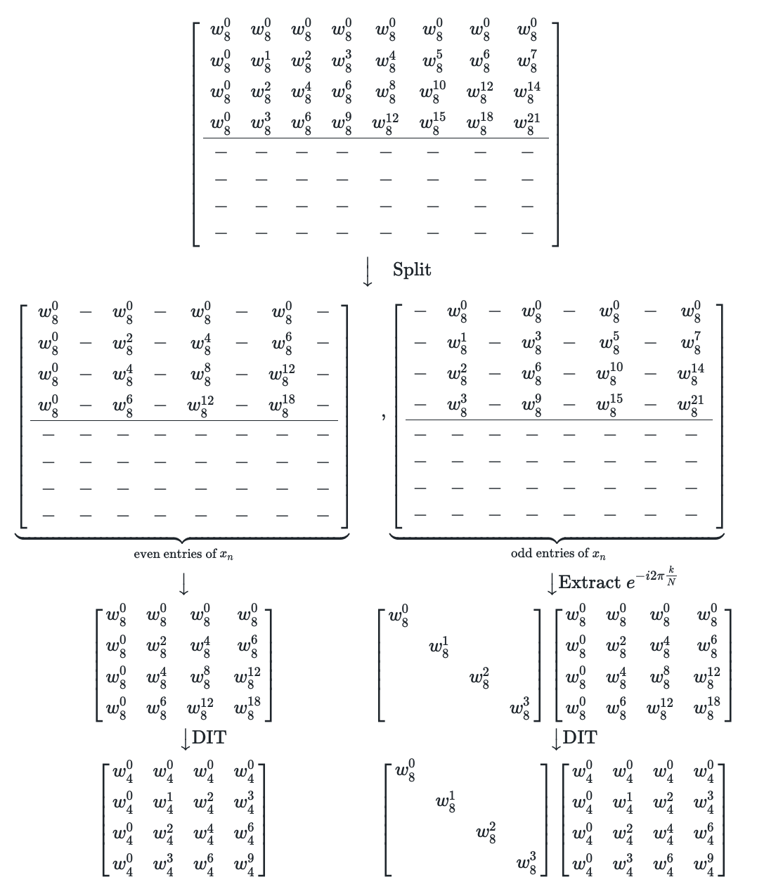
\[\begin{matrix} 0 \leq k \leq N/2: \\ \\ \\ \\ N/2 \leq k \leq N: \\ \end{matrix} \begin{bmatrix} w_8^0 & w_8^0 & w_8^0 & w_8^0 & w_8^0 & w_8^0 & w_8^0 & w_8^0\\ w_8^0 & w_8^1 & w_8^2 & w_8^3 & w_8^4 & w_8^5 & w_8^6 & w_8^7 \\ w_8^0 & w_8^2 & w_8^4 & w_8^6 & w_8^8 & w_8^{10} & w_8^{12} & w_8^{14} \\ w_8^0 & w_8^3 & w_8^6 & w_8^9 & w_8^{12} & w_8^{15} & w_8^{18} & w_8^{21} \\ \hline w_8^0 & w_8^4 & w_8^8 & w_8^{12} & w_8^{16} & w_8^{20} & w_8^{24} & w_8^{28} \\ w_8^0 & w_8^5 & w_8^{10} & w_8^{15} & w_8^{20} & w_8^{25} & w_8^{30} & w_8^{35} \\ w_8^0 & w_8^6 & w_8^{12} & w_8^{18} & w_8^{24} & w_8^{30} & w_8^{36} & w_8^{42} \\ w_8^0 & w_8^7 & w_8^{14} & w_8^{21} & w_8^{28} & w_8^{35} & w_8^{42} & w_8^{49} \\ \end{bmatrix} \\ \\ \qquad \qquad \qquad \Big \downarrow \\ \\ \begin{matrix} 0 \leq k \leq N/2: \\ \\ \\ \\ N/2 \leq k \leq N: \\ \end{matrix} \left[ \begin{array}{cccccccc} w_8^0 & w_8^0 & w_8^0 & w_8^0 & w_8^0 & w_8^0 & w_8^0 & w_8^0\\ w_8^0 & w_8^1 & w_8^2 & w_8^3 & w_8^4 & w_8^5 & w_8^6 & w_8^7 \\ w_8^0 & w_8^2 & w_8^4 & w_8^6 & w_8^8 & w_8^{10} & w_8^{12} & w_8^{14} \\ w_8^0 & w_8^3 & w_8^6 & w_8^9 & w_8^{12} & w_8^{15} & w_8^{18} & w_8^{21} \\ \hline - & - & - & - & - & - & - & - \\ - & - & - & - & - & - & - & - \\ - & - & - & - & - & - & - & - \\ - & - & - & - & - & - & - & - \\ \end{array} \right]\]The next step is to split the matrices into even and odd entries of $x_n$,
\[\left[ \begin{array}{cccc cccc} w_8^0 & w_8^0 & w_8^0 & w_8^0 & w_8^0 & w_8^0 & w_8^0 & w_8^0\\ w_8^0 & w_8^1 & w_8^2 & w_8^3 & w_8^4 & w_8^5 & w_8^6 & w_8^7 \\ w_8^0 & w_8^2 & w_8^4 & w_8^6 & w_8^8 & w_8^{10} & w_8^{12} & w_8^{14} \\ w_8^0 & w_8^3 & w_8^6 & w_8^9 & w_8^{12} & w_8^{15} & w_8^{18} & w_8^{21} \\ \hline - & - & - & - & - & - & - & - \\ - & - & - & - & - & - & - & - \\ - & - & - & - & - & - & - & - \\ - & - & - & - & - & - & - & - \\ \end{array} \right] \\ \qquad \Big \downarrow \quad \text{Split}\\ \begin{matrix} \underbrace{\begin{bmatrix} w_8^0 & - & w_8^0 & - & w_8^0 & - & w_8^0 & - \\ w_8^0 & - & w_8^2 & - & w_8^4 & - & w_8^6 & - \\ w_8^0 & - & w_8^4 & - & w_8^8 & - & w_8^{12} & - \\ w_8^0 & - & w_8^6 & - & w_8^{12} & - & w_8^{18} & - \\ \hline - & - & - & - & - & - & - & - \\ - & - & - & - & - & - & - & - \\ - & - & - & - & - & - & - & - \\ - & - & - & - & - & - & - & - \\ \end{bmatrix} }_{\text{even entries of $x_n$}} &, \underbrace{ \begin{bmatrix} - & w_8^0 & - & w_8^0 & - & w_8^0 & - & w_8^0\\ - & w_8^1 & - & w_8^3 & - & w_8^5 & - & w_8^7 \\ - & w_8^2 & - & w_8^6 & - & w_8^{10} & - & w_8^{14} \\ - & w_8^3 & - & w_8^9 & - & w_8^{15} & - & w_8^{21} \\ \hline - & - & - & - & - & - & - & - \\ - & - & - & - & - & - & - & - \\ - & - & - & - & - & - & - & - \\ - & - & - & - & - & - & - & - \\ \end{bmatrix} }_{\text{odd entries of $x_n$}} \\ \big \downarrow & \qquad \qquad \qquad \big \downarrow \text{Extract} \ e^{-i2\pi \frac{k}{N}} \\ \begin{bmatrix} w_8^0& w_8^0 & w_8^0 & w_8^0\\ w_8^0& w_8^2 & w_8^4 & w_8^6 \\ w_8^0& w_8^4 & w_8^{8} & w_8^{12} \\ w_8^0& w_8^6 & w_8^{12} & w_8^{18} \\ \end{bmatrix} & \begin{bmatrix} w_8^0 & & & \\ & w_8^1 & & \\ & & w_8^2 & \\ & & & w_8^3 \\ \end{bmatrix} \begin{bmatrix} w_8^0 & w_8^0 & w_8^0 & w_8^0\\ w_8^0 & w_8^2 & w_8^4 & w_8^6 \\ w_8^0 & w_8^4 & w_8^{8} & w_8^{12} \\ w_8^0 & w_8^6 & w_8^{12} & w_8^{18} \\ \end{bmatrix} \\ \qquad \big \downarrow \text{DIT} & \qquad \big \downarrow \text{DIT} \\ \begin{bmatrix} w_4^0 & w_4^0 & w_4^0 & w_4^0\\ w_4^0 & w_4^1 & w_4^2 & w_4^3 \\ w_4^0 & w_4^2 & w_4^{4} & w_4^{6} \\ w_4^0 & w_4^3 & w_4^6 & w_4^{9} \\ \end{bmatrix} & \begin{bmatrix} w_8^0 & & & \\ & w_8^1 & & \\ & & w_8^2 & \\ & & & w_8^3 \\ \end{bmatrix} \begin{bmatrix} w_4^0 & w_4^0 & w_4^0 & w_4^0\\ w_4^0 & w_4^1 & w_4^2 & w_4^3 \\ w_4^0 & w_4^2 & w_4^{4} & w_4^{6} \\ w_4^0 & w_4^3 & w_4^6 & w_4^{9} \\ \end{bmatrix} \\ \end{matrix}\]where the DIT stands for ‘Decimation in Time’ where we flip the $2$ in the complex exponential $\frac{2m}{N}$ down to $\frac{m}{N/2}$ which halves both the nominator and denominator, i.e. \(\begin{align} w_8^6 = e^{-i2\pi \ k \ \frac{2m}{N}} |_{m=1, k=3, N=8} = e^{-i2\pi \ k \ \frac{m}{N/2}} |_{m=1, k=3, N=8} = w_4^3 \end{align}\) Besides being mathematically correct, it makes intuitively sense, as doing $6$ steps with $1/8$’th of a stepsize is the same as doing $3$ steps with $1/4$’th of a step size on a circle.
So we obtain two DFT’s of shape $4 \times 4$,
\[\begin{bmatrix} X_0 \\ X_1 \\ X_2 \\ X_3 \\ \end{bmatrix} = \begin{bmatrix} w_4^0 & w_4^0 & w_4^0 & w_4^0\\ w_4^0 & w_4^1 & w_4^2 & w_4^3 \\ w_4^0 & w_4^2 & w_4^{4} & w_4^{6} \\ w_4^0 & w_4^3 & w_4^6 & w_4^{9} \\ \end{bmatrix} \begin{bmatrix} x_0 \\ x_2 \\ x_4 \\ x_6 \\ \end{bmatrix} + \underbrace{ \begin{bmatrix} w_8^0 & & & \\ & w_8^1 & & \\ & & w_8^2 & \\ & & & w_8^3 \\ \end{bmatrix}}_{e^{-i 2 \pi \frac{k}{N}}} \begin{bmatrix} w_4^0 & w_4^0 & w_4^0 & w_4^0\\ w_4^0 & w_4^1 & w_4^2 & w_4^3 \\ w_4^0 & w_4^2 & w_4^{4} & w_4^{6} \\ w_4^0 & w_4^3 & w_4^6 & w_4^{9} \\ \end{bmatrix} \begin{bmatrix} x_1 \\ x_3 \\ x_5 \\ x_7 \\ \end{bmatrix}\]The magic periodicity reuses the computations in the first half of the DFT to give the second half $X_{k+N/2}$ frequency bins with minimal overhead:
\[\left[ \begin{array}{} X_4 \\ X_5 \\ X_6 \\ X_7 \\ \end{array} \right] = \underbrace{ \begin{bmatrix} w_4^0 & w_4^0 & w_4^0 & w_4^0\\ w_4^0 & w_4^1 & w_4^2 & w_4^3 \\ w_4^0 & w_4^2 & w_4^{4} & w_4^{6} \\ w_4^0 & w_4^3 & w_4^6 & w_4^{9} \\ \end{bmatrix} \begin{bmatrix} x_0 \\ x_2 \\ x_4 \\ x_6 \\ \end{bmatrix} }_{\text{already computed above}} - \underbrace{ \begin{bmatrix} w_8^4 & & & \\ & w_8^5 & & \\ & & w_8^6 & \\ & & & w_8^7 \\ \end{bmatrix}}_{e^{-i 2 \pi \frac{k}{N}}} \underbrace{ \begin{bmatrix} w_4^0 & w_4^0 & w_4^0 & w_4^0\\ w_4^0 & w_4^1 & w_4^2 & w_4^3 \\ w_4^0 & w_4^2 & w_4^{4} & w_4^{6} \\ w_4^0 & w_4^3 & w_4^6 & w_4^{9} \\ \end{bmatrix} \begin{bmatrix} x_1 \\ x_3 \\ x_5 \\ x_7 \\ \end{bmatrix} }_{\text{already been computed}}\]Not using the structure of the matrix respectively the complex periodicity would have left us with a $ 8 \times 8 = 64$ matrix multiplication. Using the tricks laid out above costs us two $4 \times 4$ matrix multiplications, two $4$ additions and two $4$ multiplications for a grand total of $2 \cdot (4 \times 4) + 2 \cdot 4 + 2 \cdot 4 = 48$ operations
Upon closer inspection of the first matrix being multiplied with $[ x_0, x_2, x_4, x_6]$ we can notice that matrix exhibits the same properties and structure as the original DFT matrix. This is where the recursion kicks in in the linear algebra formulation.
For that to happen, we take the even of the evens, $[x_0, x_4]$ and the odds of the even $[x_2, x_6]$ and split them as before:
\[\text{DFT} \left( \left[ \begin{array}{} x_0 \\ x_2 \\ x_4 \\ x_6 \\ \end{array} \right] \right) = \left[ \begin{array}{} X_0 \\ X_1 \\ X_2 \\ X_3 \\ \end{array} \right] = \underbrace{ \begin{bmatrix} w_4^0 & w_4^0 & w_4^0 & w_4^0\\ w_4^0 & w_4^1 & w_4^2 & w_4^3 \\ w_4^0 & w_4^2 & w_4^{4} & w_4^{6} \\ w_4^0 & w_4^3 & w_4^6 & w_4^{9} \\ \end{bmatrix} }_{\text{yet again a DFT matrix}} \begin{bmatrix} x_0 \\ x_2 \\ x_4 \\ x_6 \\ \end{bmatrix}\]Again using the key insight that we can reconstruct the second half of the DFT bins from the first half, we can zero out a lot of computations to essentially break down the original DFT from a $4 \times 4$ to two $2 \times 2$ matrix multiplications:
\[\begin{bmatrix} X_0 \\ X_1 \\ - \\ - \\ \end{bmatrix} = \begin{bmatrix} w_4^0 & - & w_4^0 & - \\ w_4^0 & - & w_4^2 & - \\ - & - & - & - \\ - & - & - & - \\ \end{bmatrix} \begin{bmatrix} x_0 \\ - \\ x_4 \\ - \\ \end{bmatrix} + \begin{bmatrix} w_4^0 & & & \\ & w_4^1 & & \\ & & - & \\ & & & - \\ \end{bmatrix} \begin{bmatrix} - & w_4^0 & - & w_4^0\\ - & w_4^0 & - & w_4^2 \\ - & - & - & - \\ - & - & - & - \\ \end{bmatrix} \begin{bmatrix} - \\ x_2 \\ - \\ x_6 \\ \end{bmatrix}\]and we can reconfigure the already computed $2 \times 2$ matrices to get the second half of the frequency bins
\[\begin{bmatrix} X_3 \\ X_4 \\ \end{bmatrix} = \underbrace{ \begin{bmatrix} w_2^0 & w_2^0 \\ w_2^0 & w_2^1 \\ \end{bmatrix} \begin{bmatrix} x_0 \\ x_4 \\ \end{bmatrix} }_{\text{already computed}} - \begin{bmatrix} w_4^2 & \\ & w_4^3 \\ \end{bmatrix} \begin{bmatrix} w_2^0 & w_2^0\\ w_2^0 & w_2^1 \\ \end{bmatrix} \begin{bmatrix} x_2 \\ x_6 \\ \end{bmatrix}\]And we can do it yet again by observing that the $2 \times 2$ matrix can be broken up again once more (but at size 1 the recursion naturally stops). Similarly this recursion applies equally to the original odd entry terms in the upper most recursion layer.
This recursive breaking up matrices and saving half the computations (via reconstruction of the second half of the frequency bins) gives the FFT its highly useful $O(N \log N)$ complexity.
The efficiency stems from us retracing the recursive matrix break ups with our results once we arrived at the DFT with length of one. Each evaluation in the recursion allows us to reconstruct frequency bins twice our original size (thanks to periodicity) with minimal overhead, which goes from $1 \rightarrow 2 \rightarrow 4 \rightarrow 8$. So for signals of length $8$, we need 4 recursive step to arrive at a DFT length of one, from which we can reconstruct the frequency bins efficiently. For a signal of length $16$ we need 5 recursions, for $32$ just one more, namely 6 recursions, and for $64$ just seven recursions. While the speed up might be small for short signals, audio people with 20.000 samplings steps should seriously rejoice and feel blessed by the $O(N \log N)$ complexity.
The inverse DFT
In order to reconstruct a signal from its Fourier coefficients $X_k$, we multiply the frequency amplitude $X_k$ with a complex exponential which is a periodic function with a specific frequency $k$. We have the reconstruction \(x_n = \frac{1}{N} \sum_{k=0}^K X_k e^{i 2\pi k \frac{n}{N}}\)
where the only difference to the DFT is the minus sign in the exponential and a scaling factor $1/N$. The cool thing is that the minus sign has no influence on the core structure of the transformation, so we can employ the entire algorithm again for the reconstruction from frequency to time domain.
Thus we have a $O(N \log N)$ algorithm both for the transformation in both directions. Sweet …