The Weight of Sampling

Why we need it

Suppose you want to estimate $\mathbb{E}_p[f(X)]$ for some target distribution $p$. In a perfect world, you’d draw $N$ i.i.d. samples from $p$ and compute the sample mean. The variance of that estimator drops as $1/N$ — that’s what you learn in ML 101.

If we can draw i.i.d. samples from $p$, then there’s no real problem in computing the expectation. But alas, we can’t always draw i.i.d. samples from $p$.

But sampling from $p$ is not always possible. This can be for a variety of reasons, but one common reason is that the distribution $p$ is complex and high-dimensional and it’s normalization constant is not known. Oftentimes, we only know $p$ up to a normalizing constant $p = \tilde{p} / Z$. Without knowing $Z$, we can’t assign the correct probability to a point $x$ under $p(x)$. For the same value of $\tilde{p}(x)$, the probability of $x$ under $p(x)$ is different if $Z$ is different.

The mathematical version of this predicament shows up everywhere. Consider the workhorse of modern machine learning: Bayesian posterior inference. You observe data $\mathcal{D}$ and want to reason about parameters $\theta$ under the posterior

The numerator — likelihood times prior — you can evaluate pointwise, no problem. But the denominator $p(\mathcal{D})$, the marginal likelihood, requires the probability of your entire dataset $\mathcal{D}$ under the model.

So either you somehow magically know the probability of every sample in your dataset $\mathcal{D}$ under the model, or you need to estimate it by defining every possible value of $\theta$ and evaluating the likelihood and prior for each of them. Every possible vaue of $\theta$ for continuous parameters is an infinite number of values, so you’d need an infinite amount of computational resources to evaluate the likelihood and prior for each of them.

For anything beyond toy conjugate models, this integral is intractable: there is no closed-form solution and the dimensionality of $\theta$ makes brute-force numerical integration hopeless. So you’re stuck with a distribution you can evaluate (up to a constant) but can’t sample from directly. You know the shape of the landscape, but you have no way to generate points that are distributed according to it.

This is where sampling schemes come in. But in practice, the samples these schemes produce are almost never i.i.d. from the target:

• MCMC produces samples that are serially correlated (each sample depends on the previous one).
• Importance sampling draws from a proposal $q \neq p$, then corrects with weightsf — but those weights can be wildly uneven.
• Particle filters resample with replacement, creating duplicate particles.

All of these schemes are ways to sample from $p$ even if you can’t sample from $p$ directly. In all these cases, your $N$ raw samples carry less information than $N$ truly independent samples from the OG $p$ would. You need a single number that answers: “how many i.i.d. samples is my collection of samples I proposed actually worth?” That number is the ESS.

Without it, you’re flying blind — you can’t meaningfully compare algorithms, diagnose poor mixing, set stopping criteria, or calibrate your confidence in Monte Carlo estimates.

Let’s get the equations rolling

Importance Sampling

We want to compute:

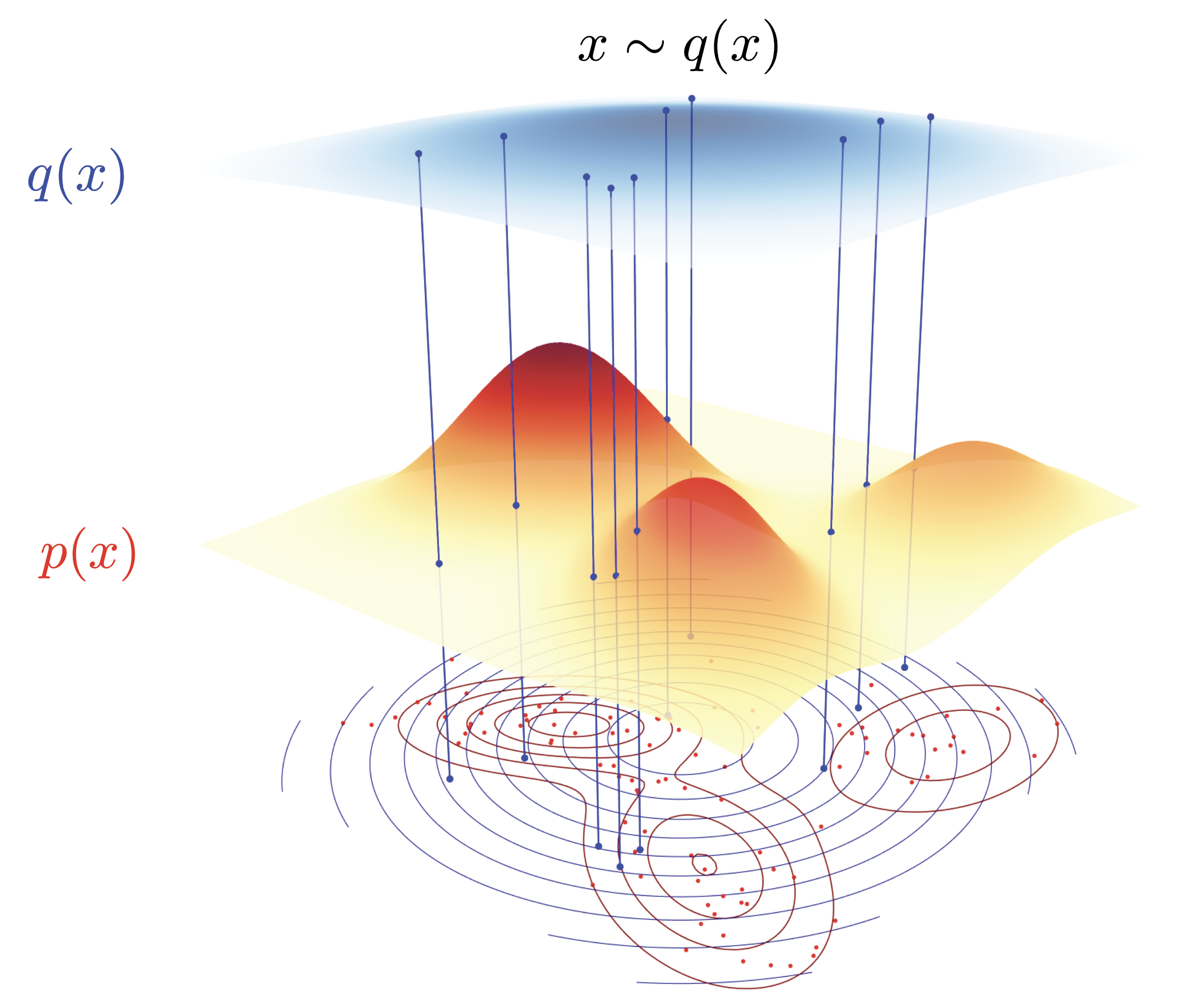
We can’t sample from $p$ directly, so we draw $X_1, \dots, X_N \overset{\text{i.i.d.}}{\sim} q$ from a proposal distribution $q$, and use the importance sampling identity:

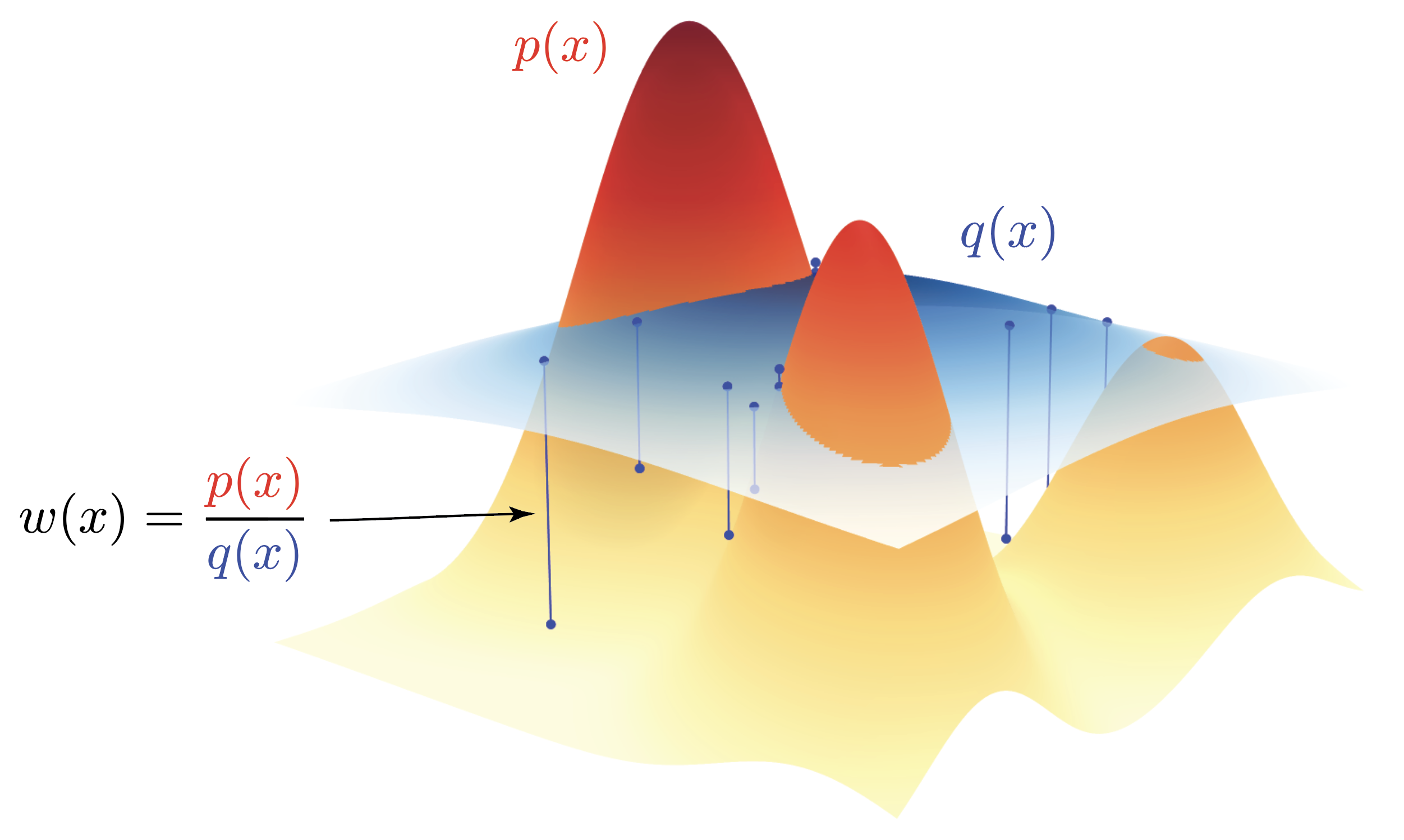
where $w(x) = p(x)/q(x)$ are the (unnormalized) importance weights.

Below you can see the importance weights $w(x) = p(x)/q(x)$ for a Gaussian mixture model from the cover. If we sample from $q$ we have to take into consideration that we’re not sampling from $p$ directly. The correction for sampling from $q$ but wanting to estimate the expectation under $p$ is given by the importance weights $w(x) = p(x)/q(x)$. For all examples in the visualization below, $p(x) < q(x)$, such that th importance weights will all be smaller than 1. These weights $w(x) < 1$, will thus downweight the contribution of the samples from $q$ in the expectation estimator,

whereas parts where $p(x) > q(x)$, the importance weights will be greater than 1, thus upweighting the contribution of the samples from $q$ in the expectation estimator.

Deriving the self-normalized estimator

The problem with standard importance sampling

If we know $p$ exactly (including its normalizing constant), life is simple. The standard IS estimator is:

This is unbiased:

But in practice — especially in Bayesian inference — we only know $p$ up to a normalizing constant $p = \tilde{p} / Z$. While we’re interested in estimating $w = p / q$, we’re left holding the bag with it’s unnormalized cousin where $Z$ is unknown,

which makes us arrive again at the same spot we started from that we don’t know $Z$ in the first place. But with unnormalized weights $\tilde{w}$, there is a trick we can pull to bootstrap ourselves out of this seemingly dead end.

The key observation is that the normalizing constant $Z$ is itself is an integral over the whole space $x$ of $\tilde{p}(x)$. We can therefore use importance sampling to evaluate the integral as in

Given that we’ve generated the samples $x \sim q$ proportionally to the distribution $q$ by definition, the expectation reduces to a simple average over the samples $x$,

Going back to our original objective we want to identify

Whereas the importance estimator \(\hat{\mu}_{\text{IS}}\) assumes access to the target distribution $p$ including its normalization constant $Z$, using the unnormalized weights \(\tilde{w}\) to estimate \(\hat{Z}\) turns this estimator it to the self-normalized estimator \(\hat{\mu}_{\text{SN}}\).

We can simplify the equation for $\hat{\mu}_{\text{SN}}$ even further by observing that the sum in the denominator is self contained (as in sum over $j$), so we can write

where the normalized weights $\bar{w}$ are defined as

How much does our estimator actually vary?

The self-normalized estimator $\hat{\mu}_{\text{SN}}$ is a ratio of two random quantities. This makes its variance analysis more subtle than the simple i.i.d. case.

The key question is: how much does our estimate vary from one set of samples to the next? If we draw $N$ samples from $q$ repeatedly, how much will $\hat{\mu}_{\text{SN}}$ fluctuate around the true mean $\mu$?

Here’s a (somewhat) intuitive example: Let’s assume we want an estimate of the average height of people in Europe by sending $N$ random people a text message. Imagine you picking 100 random cell phone numbers and blasting off a text saying “Yo, how tall are you?”. These text message could arrive on a Greek island in the sun, in the eternal winter darkness of a Finnish village or in the land of the giants, Holland.

Problem is, you don’t know how tall nor how representative the person reading the text is for the average height of people in Europe. Ideally, you want to representatively sample from all countries in Europe from all height groups: the small people in Holland, the tall and small people in Portugal and the average tall people in Greece.

The variance of your little survey depends on two factors:

1. The intrinsicly different heights in Europe that exists regardless of who you pick. Every country has differently tall people.
2. Who you send the text to in Europe from your 100 allowed text messages.

Particularly the second source of variability is tricky in our case. Did you send the text message it by accident to all Dutch men measuring 2.14m? Then your average is like 2.05m. Hardly realistic. Or maybe you send it to all Greek grandmas towering at a mighty 1.55m. Also hardly representative.

In more mathy terms we would say that the variance of $\hat{\mu}_{\text{SN}}$ depends on two factors:

1. The intrinsic variability of $f(X)$ under the target distribution $p$ captured by $\sigma_f^2 = \text{Var}_p[f(X)]$. (the natural distribution of heights in Europe)
2. The mismatch between proposal $q$ and target $p$, reflected in the weight variability. ($q$ being the proposed people you send your height text message to)

When $q$ is a poor approximation to $p$, a few samples will have very large weights while most have tiny weights. For simplicites sake assume that $q$ is a uniform $q=1/100$. The probability of picking the tiny Greek grandmas or the super tall male Dutchies is very small as their heights are at the far ends of the height distribution in Europe. The average height is around 1.75m, so picking a height of 1.55m or 2.14m is very unlikely.

It’s important to note that we’re self-normalizing the weights $\tilde{w}_i$ with all our samples, so we have \(\bar{w}_i = \tilde{w} / \sum_{j=1}^{100} \tilde{w}_j\).

If we ask 98 Greek grandmas and towering Dutchies and only 2 slightly less extreme samples, the contribution of those extreme 98 weights will be negligible. Remember that in order to compute the average weight we’ll compute,

But lo and behold, due to $p$ being very small, the weights of the 98 unrepresentative samples have a negligible contribution to the overall value. In effect, we’re trying to estimate the average European height with two samples. Not ideal when we had assumed that we used 100 samples.

This weight concentration in those two meaningful samples means we’re effectively using far fewer than $N$ samples, inflating the estimator variance. The effective sample size (ESS) quantifies exactly how many “equivalent i.i.d. samples” our weighted samples represent. In our case it’s two, not a hundred.

But how do we quantify this effetive sample size?

The Variance of our Estimator

Let’s denote the number of effective samples as $N_{\text{eff}}$.

If we had $N$ i.i.d. samples from $p$, the variance of the sample mean would be:

where $\sigma_f^2 = \text{Var}_p[f(X)]$.

But alas, we don’t have access to samples from $p$ because if we had, I wouldn’t have to write this blog post explaining ESS.

What we do have is our estimator $\hat{\mu}_{\text{SN}}$,

The variance is easy to set up, but actually a bit tricky to compute analytically as we’re dealing with a ratio of random variables

The Delta Method (or “Everybody’s Favourite Tool: Linearization with Taylor Expansions”)

Imagine you have two random variables, say $X$ and $Y$, and you care about the ratio $g(X, Y) = X/Y$. You know the variances and covariance of $X$ and $Y$, but what’s the variance of the ratio? That’s awkward because the ratio is nonlinear — variances don’t just “pass through” nonlinear functions.

The delta method’s trick is simple. All we gonna do is locally linearize the function via a first-order Taylor expansion around the means, then compute the variance of that linear approximation. Since variance behaves nicely under linear transforms, you get a clean closed-form result (albeit be it an only locally valid result due to the linearization).

Let $g(X, Y) = X / Y$.

Let’s start with the one-dimensional case to build intuition. The Taylor expansion of a smooth function $g(X)$ around a point $\mu_X$ is:

Now let’s extend this to two dimensions. The exact formula is actually bit complicated for the infinite sum but the practically interesting parts are

Only using the first order yields the truncated version in the form of

For the delta method, we keep only the first-order term (linearization):

Taking the variance of both sides (and noting that $\mu_X , \mu_Y$ is a constant so $\mathbb{V}[\mu_X] = \mathbb{V}[\mu_Y] = 0$), we have

where the last term $\mathbb{C}[X, Y]$ is the covariance between $X$ and $Y$ as they might or might not be correlated.

The required partial derivatives are:

Substituting:

Naturally, this approximation degrades when $\mu_Y$ is close to zero since we’re effectively dividing by something close to zero or when the distributions have heavy tails. In ML contexts (e.g., variance of a metric ratio in A/B testing), if our samples are large enough for CLT to kick in, this works extremely well.

For our case, we would have

Linearizing the Ratio in the Variance Estimator

For the linearization to be applicable we need the expected values and the variances of the nominator and denominator in our self-normalizing importance sampler.

First up we need to compute the mean and the variance of nominator and denominator

All of the expectations and variances above are with respect to a random variable $X$ and it’s functions $\tilde{w}(X)$ or $f(X)$. The expectation and variance operator are both linear for a sum of random variables, so we can generically write

For the covariance calculation we’ve exploited the fact that over $N$ samples, we assume that only samples with the same index are correlated, whereas samples with different indices are independent.

Since the terms in $\mathbb{V}[X/Y]$ are all variances, we have to simply add a $1/N$ factor to each term, if we choose to work with the sum instead of the mean. In any case, since the $1/N$ factor can be inserted in both the nominator and denominator, it won’t change the final result anyway.

Putting all of these terms together we get

The equation above is an approximation of the variance of the self-normalized estimator. If we sample the samples from a proposal distribution $q$ that is different from the unnormalized target distribution $\tilde{p}$ resulting in the weights $\tilde{w}$.

But what if we wouldn’t sample from $q$ but from the true target distribution $p$ resulting in the weights $w$? This implies that we can really generate $N_p$ samples from $p$ directly, and thus our samples will be i.i.d. from $p$, not suffering from the approximation error of $q$ to $p$. Let’s calculate the variance of the self-normalized estimator if we were to sample from $p$ directly,

And thus we can see that the variance is actually decreasing with the number of samples $N_p$ from $p$ directly as we would expect from a standard i.i.d. estimator. If $N_p$ is large, we consequently decrease the inherent variance of the estimator by a factor of $N_p$.

But again, we can only sample from $q$, not from $p$. But we can pose a clever question: How many samples $N_q$ from $q$ would we need to get the same variance as $N_p$ samples from $p$? At the very beginning we said that our correlated samples from $q$ carry less information than $N_p$ truly independent samples would. So the ESS metric asks the question how many samples $N_q$ from $q$ are worth $N_p$ perfect, i.i.d, super-duper-excellent samples from $p$?

In order to solidify this, we’ll set the two variance estimators equal to each other, one with $N_p$ samples and one with $N_q$ samples. \(\begin{align*} \mathbb{V}_p\left[\frac{\sum \tilde{w} \ f}{\sum \tilde{w}}\right] &= \mathbb{V}_q\left[\frac{\sum \tilde{w} \ f}{\sum \tilde{w}}\right] \\ \frac{1}{N_p} \mathbb{E}_p\left[ \ \left( f - \mu_f\right)^2\right] &= \frac{1}{N_q} \frac{\mathbb{E}_q\left[ \tilde{w}^2 \ \left( f - \mu_f\right)^2\right]}{\mathbb{E}_q[\tilde{w}]^2} \\ \end{align*}\)

In order to arrive at the ESS formula, we’ll need to do a final approximation by assuming that the weights $\tilde{w}^2$ actually aren’t too correlated with $(f - \mu_f)^2$ which is in practice actually somewhat true,

The samples $N_q$ are then the effective number of samples from $q$ that are worth $N_p$ samples from $p$. The ratio $\frac{\mathbb{E}_q\left[ \tilde{w}^2 \right] }{\mathbb{E}_q[\tilde{w}]^2}$ can intuitively be interpreted as a discount factor. You can quite literally think of the discount factor like a conversion rate between the number of samples from $q$ and the number of samples from $p$ that are worth the same. This really akin to conversion factors between currencies. Take $N_q$ Zimbabwen dollars and try to convert them to $N_p$ US dollars. Since Zimbabwen dollars aren’t worth anything, you got like 0.000001 Dollar per Zimbabwen dollar. So you need an inordinate amount of Zimbabwen dollars to get a single $N_p=1$ US dollar.

We can also express the effective sampling size in terms of normalized weights $\tilde{w}$ instead of $\tilde{w}^2$. Remember that

This gives us an easy way to calculate the ESS purely from the normalized weights $\tilde{w}_i$.

MCMC

In the importance sampling case, the problem was that we couldn’t sample from $p$ and had to use a proposal $q$, leading to weights that could be wildly uneven. MCMC flips the script entirely: we are sampling from $p$ (at least asymptotically), but our samples are serially correlated because each sample depends on the previous one.

Think of it this way: if importance sampling suffers from “some samples mattering way more than others”, MCMC suffers from “consecutive samples being almost the same thing”. You’re walking through the mountainous landscape we described at the very beginning, but you can only take small steps from where you currently are. If you’re standing on a peak, your next few hundred positions will all be near that same peak — you haven’t explored the valleys yet. Your chain might eventually visit the entire landscape, but locally, your samples are redundant.

So the question is the same one we’ve been asking all along: how many i.i.d. samples is our correlated chain actually worth?

Let’s set up the math. Denote the sample mean of our MCMC chain as

where $X_1, X_2, \ldots, X_N$ are the states of our Markov chain targeting $p$.

We want $\mathbb{V}[\bar{f}_N]$. Let’s expand this directly from the definition:

Now here’s where the correlation makes life interesting. What we’ve done is run a MCMC chain which always takes the last value $X_{t-1}$ as the starting point for the next step $X_t$. So for all intents and purposes, the samples $X_t$ are correlated. The variance of a sum is not just the sum of the variances when the summands are correlated. We have to account for all the cross-terms:

This is a double sum — every pair of samples $(t, s)$ contributes a covariance term. The diagonal terms ($t = s$) give us the familiar sum of variances, while the off-diagonal terms ($t \neq s$) capture the correlations between different samples. For i.i.d. samples, all the off-diagonal terms vanish because $\mathbb{C}[f(X_t), f(X_s)] = 0$ for $t \neq s$, and we’d recover

But for MCMC, they don’t vanish. Consecutive samples are correlated, and that correlation bleeds into the variance.

The saving grace is stationarity: if you run the chain long enough after which the chain is said to have “converged”, the covariance between $f(X_t)$ and $f(X_s)$ depends only on the lag $k = |t - s|$, not on the absolute positions $t$ and $s$. With stationarity, this allows us define the autocovariance function:

Note that $c_0 = \sigma_f^2$ (the marginal variance of $f$ under $p$, the same $\sigma_f^2$ we’ve been carrying around since the beginning) and $c_k = c_{-k}$ by symmetry — the covariance doesn’t care about the direction of time.

In the double sum $\sum_{t=1}^N \sum_{s=1}^N$, we need to count how many pairs $(t, s)$ produce each lag $k = t - s$. This is a straightforward combinatorial exercise:

• Lag $k = 0$: pairs $(1,1), (2,2), \ldots, (N,N)$ → exactly $N$ terms
• Lag $k = 1$: pairs $(2,1), (3,2), \ldots, (N, N-1)$ → exactly $N-1$ terms
• Lag $k = -1$: pairs $(1,2), (2,3), \ldots, (N-1, N)$ → exactly $N-1$ terms
• In general, lag $k$: exactly $N - |k|$ terms, for $k = -(N-1), \ldots, N-1$

This allows us to simplify the equation as for any fixed $k=t-s$, there are $N - |k|$ pairs $(t, s)$ that produce this lag with a fixed value of $c_k$ for the stationary/converged chain. So the double sum collapses to

Using the symmetry $c_k = c_{-k}$, we fold the negative lags into the positive ones:

Plugging this back into our variance expression:

Defining the autocorrelation function $\rho_k = c_k / c_0$ (the normalized version of the autocovariance), we arrive at

For i.i.d. samples, $\rho_k = 0$ for all $k \geq 1$, and the bracket collapses to $1$, recovering the familiar $\sigma_f^2/N$ we know and love.

The Bartlett weights $(1 - k/N)$ are worth pausing on. They arise purely from counting: at lag $k$, there are only $N - k$ pairs of samples separated by exactly $k$ steps. The further apart two samples are in the chain, the fewer such pairs exist. For large $N$, these weights are approximately $1$ for any fixed lag — the edge effects wash out.

Thus for large $N$, the Bartlett weights $(1 - k/N) \to 1$ for any fixed $k$. If the autocorrelations decay fast enough that $\sum_{k=1}^\infty \|\rho_k\| < \infty$ — which holds for any geometrically ergodic chain, i.e. pretty much every well-behaved MCMC sampler you’ll encounter in practice — we can take the limit:

where we’ve defined the integrated autocorrelation time (IAT):

The name “integrated” comes from viewing this as the discrete analogue of integrating the continuous autocorrelation function. It collapses the entire memory structure of the chain into a single number.

What does $\tau_f$ tell us?

• $\tau_f = 1$: no autocorrelation at all, we’re back in i.i.d. land because all $\rho_k = 0$ for $k \geq 1$
• $\tau_f = 10$: each sample carries only $1/10$-th the information of an independent draw
• $\tau_f = 100$: the chain is mixing like molasses — you need 100 steps to get one effective independent sample

One subtlety worth flagging: notice the subscript $f$ on $\tau_f$. Unlike the importance sampling ESS we derived above — which is purely a function of the weights and therefore the same no matter what $f$ you’re estimating — the MCMC IAT is function-dependent. A chain might mix quickly for the mean of $f$ but slowly for its variance, or zip along in one direction of parameter space while crawling in another. This is a fundamental difference between the two flavors of ESS.

We now play exactly the same game as in the importance sampling case. We ask: how many i.i.d. samples $N_{\text{eff}}$ from $p$ would give us the same variance as our $N$ correlated MCMC samples?

The i.i.d. baseline is, as before:

Setting this equal to the MCMC variance:

The $\sigma_f^2$ cancels — though this is a bit misleading, since $\tau_f$ itself depends on $f$, so the ESS is still function-dependent unlike the IS case:

The logic is beautifully parallell to what we did for importance sampling. There, the “discount factor” was the weight variability $\mathbb{E}_q[\tilde{w}^2] / \mathbb{E}_q[\tilde{w}]^2$. Here, the discount factor is the integrated autocorrelation time $\tau_f$. Both tell you how many of your $N$ samples you’re actually using.

Going back to our currency analogy: if importance sampling was converting Zimbabwean dollars to US dollars (with the exchange rate determined by weight concentration), then MCMC is like converting a time series of correlated price observations to independent ones (with the exchange rate determined by how sticky the prices are). Either way, you’re asking: what’s my real purchasing power?

Diffusion Models as Sequential Monte Carlo

We’ve now built up the entire ESS toolkit: for importance sampling, it measures weight concentration; for MCMC, it measures autocorrelation-induced information loss. These two stories converge in one of the most consequential generative modeling frameworks of the last few years — diffusion models — where the denoising process can be interpreted as a sequential Monte Carlo sampler.

But before we get to diffusion models, let’s set up the general SMC framework. The whole point of SMC is to do inference in state-space models (also known as hidden Markov models in the discrete case), where we have:

• A sequence of hidden states $x_0, x_1, \ldots, x_T$ that we can’t observe directly
• A prior over the initial state: $p(x_0)$
• A transition kernel $p(x_t | x_{t-1})$ describing how the hidden state evolves over time
• An emission model (also called the observation model) $p(y_t | x_t)$ describing how the observed data $y_t$ is generated from the hidden state

The joint distribution over the full trajectory and observations factorizes as

The goal is to compute the filtering distribution $p(x_t | y_{1:t})$ — what do we believe about the current hidden state, given everything we’ve observed so far? — or, more ambitiously, the smoothing distribution $p(x_{0:T} | y_{1:T})$ over the entire trajectory.

The emission probability $p(y_t | x_t)$ is the likelihood of the observed data $y_t$ given the hidden state $x_t$. In effect, it works as a critic of the trajectory $x_{0:t}$ that was sampled so far. At each step (but also maybe only at other steps) it evaluates the probability $p(y_t | x_{0:t})$ of the observed data $y_t$ given the trajectory $x_{0:t}$. If you did a lot of steps that moved your samples $x_t$ into some part of space where the data $y_t$ is very unlikely, your weight will be low, and thus that particular sample path $x_{0:t}$ will be highly discouraged.

The trouble is that the corresponding analytical posteriors are intractable in general. The exact recursion involves integrating over all possible previous states at every step, and this integral doesn’t have a closed form except in special cases (linear-Gaussian dynamics give you the Kalman filter; finite state spaces give you the forward-backward algorithm).

Sequential Monte Carlo approximates these intractable distributions using a weighted set of particles — sample trajectories ${x_{0:t}^{(i)}, w_t^{(i)}}_{i=1}^N$ that represent an empirical approximation to the posterior. The algorithm proceeds sequentially:

1. Propagate: Move each particle forward in time by sampling from the transition kernel $x_t^{(i)} \sim p(x_t | x_{t-1}^{(i)})$
2. Weight: Assign each particle an importance weight based on the emission model $\tilde{w}_t^{(i)} = p(y_t | x_t^{(i)})$
3. Normalize: Compute $\bar{w}_t^{(i)} = \tilde{w}_t^{(i)} / \sum_j \tilde{w}_t^{(j)}$
4. Evaluate: Compute the ESS $\hat{N}_{\text{eff}} = 1 / \sum_i (\bar{w}_t^{(i)})^2$
5. Resample: If the ESS drops below a threshold, resample particles according to the weights — duplicate the promising ones, discard the dead weight — and reset all weights to $1/N$

Essentially, you keep sampling trajectories and you keep using the “critic” to evaluate them by checking what the probability is that the trajectory would have produced the data $y_t$ that you observed. This information is encapsulated in the weights $w_t^{(i)}$ that you assign to each trajectory. If the weights become too low, this implies that your trajectories have become more and more unlikely for the “critic” $p(y_t | x_{0:t})$. What do you do? You look at your trajectories and you decide to keep only the ones that are still likely, and you discard the ones that are not. The normalized weights $\bar{w}_t^{(i)}$ can then be used as the probabilities for a categorical distribution that you use to sample new trajectories.

Now — what does any of this have to do with diffusion models?

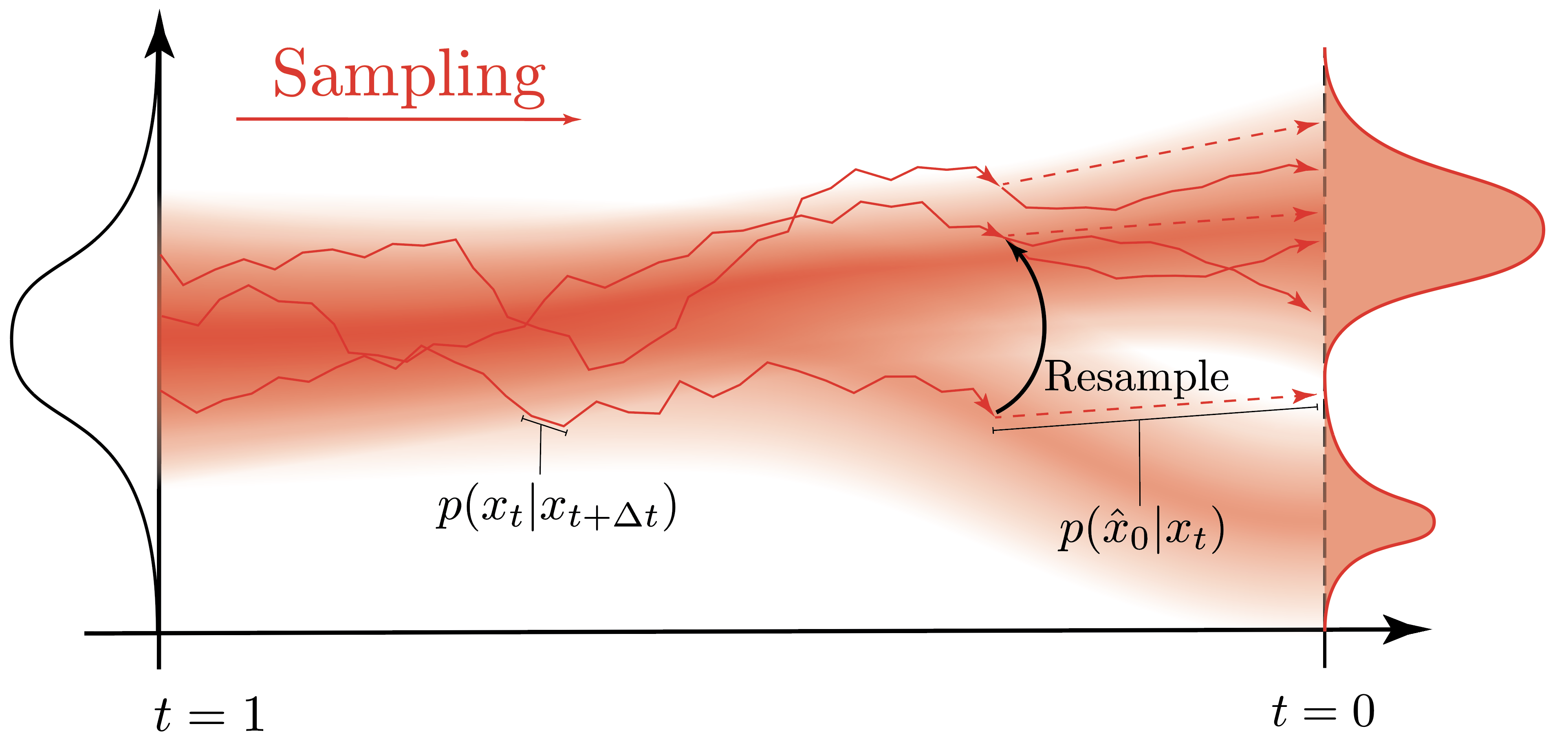
For diffusion models, we have the generative reverse-time SDE:

where $W_t$ is a reverse-time Wiener process and $\nabla_{x_t} \log p_t(x_t)$ is the score function — the gradient of the log-density at time $t$. This is the quantity a diffusion model learns: a neural network $s_\theta(x_t, t) \approx \nabla_{x_t} \log p_t(x_t)$.

To actually generate samples, we discretize the reverse SDE with an Euler-Maruyama step of size $\Delta t$:

This discretization is our transition kernel — reading it off as a Gaussian:

This is the transition kernel that enters the SMC framework. Unconditional generation is then straightforward: sample $x_T \sim \mathcal{N}(0, I)$, apply $p_\theta(x_{t-\Delta t} | x_t)$ for each step backwards, and out pops a sample $x_0 \approx p_{\text{data}}$. This is just a Markov chain — no weights, no resampling, no ESS to speak of.

The one-step denoiser: Tweedie’s formula

Before we get to SMC, we need one more ingredient: the “critic” $p(y_t | x_t)$. At any noise level $t$, the diffusion model implicitly gives us a one-step denoiser — a direct estimate of what the clean data $x_0$ looks like, given only the current noisy state $x_t$.

This comes from Tweedie’s formula. Given the forward marginal $q(x_t | x_0) = \mathcal{N}(x_t;\, \alpha(t)\, x_0,\, \sigma^2(t)\, I)$, the posterior mean of $x_0$ given $x_t$ is:

Since the diffusion model learns the score $s_\theta(x_t, t) \approx \nabla_{x_t} \log p_t(x_t)$, we get $\hat{x}_0(x_t)$ essentially for free — it’s just a different way of reading off the network output.

Think of $\hat{x}_0(x_t)$ as the model’s best guess of the clean image, peeking through the noise at step $t$. Early in the denoising process (large $t$, lots of noise), this guess is blurry and uncertain. Late in the process (small $t$, little noise), it’s sharp and confident.

We’ll call this one-step denoiser prediction the “observation” that the current noisy state $x_t$ produces — and denote the observation model as $p(y_t | x_t)$, where $y_t$ encodes what we can infer about the data from $x_t$.

Conditional generation: enter the state-space model

Now suppose we don’t just want any sample from $p_{\text{data}}$ — we want a sample that satisfies some condition $y$. Maybe we want an image of a golden retriever, or we want to inpaint a missing region, or we want a molecule with certain properties.

What we want is to sample from the conditional reverse process:

The problem? The likelihood $p(y | x_0)$ only tells us about the final clean sample $x_0$. We don’t get any signal about whether our denoising trajectory is heading in the right direction until the very end. By then, it’s too late — all our computational budget is spent.

This is where the one-step denoiser saves the day. Instead of waiting until $x_0$ to evaluate $p(y | x_0)$, we can get an approximate per-step likelihood using the Tweedie estimate:

We’re peeking at the model’s current best guess of the clean output and asking: “does this look like it satisfies the condition?”

And now we have all the pieces to write down a state-space model — exactly the structure we introduced in the general SMC framework above:

• Hidden states $x_T, x_{T-\Delta t}, \ldots, x_0$ — the noisy latents at each denoising step
• Prior $p(x_T) = \mathcal{N}(0, I)$ — pure noise at the start of the reverse process
• Transition kernel $p_\theta(x_{t-\Delta t} \| x_t)$ — the Euler-Maruyama discretization of the reverse SDE
• Emission model $p(y_t | x_t) \approx p(y | \hat{x}_0(x_t))$ — how consistent is the current state with the desired condition, as estimated through the one-step denoiser

This is exactly the structure we need for a particle filter.

Combining everything we get the following algorithm:

Initialize: Draw $N$ particles from the prior (pure noise):

For each denoising step $t = T, T-\Delta t, \ldots, \Delta t$:

1. Propagate each particle through the transition kernel (one reverse SDE step):

2. Compute the unnormalized importance weights via the observation model:

The weight of each particle reflects how well its one-step denoiser prediction $\hat{x}_0(x_t^{(i)})$ matches the desired condition $y$.

3. Normalize the weights:

Look familiar? These are exactly the self-normalized weights $\bar{w}_i = \tilde{w}_i / \sum_j \tilde{w}_j$ we spent the first half of this post deriving.

4. Compute the ESS using the formula we derived:

5. Resample if necessary: if $\hat{N}_{\text{eff}}$ drops below some threshold (a common choice is $N/2$), resample the particles according to the weights — duplicate the high-weight particles and discard the low-weight ones. After resampling, reset all weights to $1/N$ and continue denoising from the refreshed particle cloud.

Why ESS matters here: the weight degeneracy problem

And here’s where our entire ESS derivation pays off.

Remember the Dutch giants and Greek grandmas? In the diffusion context, the particles are like our text message recipients. Each particle $x_t^{(i)}$ is a different “hypothesis” for what the clean image looks like. Some particles, by chance, will be heading toward images that satisfy the condition $y$ — samples that score highly under the observation model. Others will be heading toward something completely different: samples that bear no resemblance to the desired condition, effectively dead weight in the particle cloud.

The weights $\tilde{w}_t^{(i)} = p(y | \hat{x}_0(x_t^{(i)}))$ quantify this mismatch: particles whose one-step denoiser prediction aligns well with the condition $y$ get large weights, while those drifting toward irrelevant regions of the sample space get negligible weights. If only 2 out of 100 particles are heading in the right direction, the ESS will be approximately 2 — just like our Dutch-and-Greek height survey.

Without resampling, the particle cloud degenerates: a handful of particles carry all the weight, and you’re effectively running the denoising process with just those few trajectories. The estimator variance explodes, and the quality of your conditional samples plummets.

Resampling — triggered when the ESS drops below a threshold — is the remedy. It prunes the dead-weight particles and replicates the promising ones, refreshing the particle cloud. But the price is that resampled particles are no longer independent (they share common ancestors), introducing the autocorrelation that we analyzed in the MCMC section. So we’re back to our old friend: correlated samples carrying less information than independent ones.

This is the fundamental tension of SMC: resampling fights weight degeneracy but creates sample correlation. The ESS, in both its importance-sampling and MCMC flavors, is the diagnostic that navigates this tradeoff.

Deriving the incremental weights

So far we have the transition probabilities $p_\theta(x_{t-\Delta t} | x_t)$ — the reverse SDE that propagates our particles from noise toward data. But transitions alone just tell us how particles move; they say nothing about which particles are worth keeping. For that, we need the emission probabilities $p(y_t | x_t)$.

The idea is simple: we define a function that takes in a particle $x_t$ and returns a scalar value evaluating how well that particle’s trajectory aligns with the desired observation $y$. In the diffusion setting, we use the one-step denoiser to peek ahead: $p(y_t | x_t) \approx p(y | \hat{x}_0(x_t))$. This is our critic — it scores each particle at time $t$ by asking “if I were to denoise this particle all the way to $x_0$ right now, how well would the result match the condition $y$?”. In the literature, this is often called the “potential function” and denoted by the function $G_t(x_t)$.

The whole point of tracking importance weights is to keep score of which samples are good and which are bad, so that we can resample accordingly — duplicate the promising trajectories and prune the hopeless ones. And for that resampling decision to be well-informed, we need the most up-to-date emission probability at every time step $t$, not just at the very end.

We can achieve exactly this with a telescoping product. Define the per-step potential function $G_t(x_t)$:

This is the ratio of the current emission score to the previous one — how much our assessment of the particle has changed in a single denoising step. Remember, we’re going from $T \to 0$, so the previous step is $t + \Delta t$. If the particle is making progress toward satisfying the condition, $G_t > 1$ and the weight increases. If it’s drifting away, $G_t < 1$ and the weight decreases. The incremental unnormalized importance weight at step $t$ is then simply

Now watch what happens when we accumulate these incremental updates. The denominators and numerators of consecutive steps cancel each other:

since $\hat{x}_0(x_0) = x_0$ (fully denoised) and $p(y | \hat{x}_0(x_T))$ is essentially constant — pure noise carries no information about $y$. The telescoping gives us the best of both worlds: at any point in time $t$, the accumulated weight reflects the most up-to-date emission probability $p(y | \hat{x}_0(x_t))$, while the recursive update via $G_t$ means we only ever need to compute a single ratio per step (instead of keeping track of the entire trajectory).

The big picture

Let’s step back and admire the view from the top of this particular mountain. What we’ve shown is that conditional diffusion generation is, at its core, a particle filter:

• The prior $p(x_T) = \mathcal{N}(0, I)$ is where our particles start: pure isotropic noise.
• The transition kernel $p_\theta(x_{t-\Delta t} | x_t)$ — the discretized reverse SDE — propagates particles toward cleaner states.
• The emission model $p(\hat{x}_0 | x_t)$ evaluates each particle’s one-step denoiser prediction against the desired condition.
• The importance weights $\tilde{w}_t$ measure how well each particle’s denoised prediction matches $y$.
• The ESS — computed as $1/\sum_i \bar{w}_i^2$ — tells us how many particles are effectively contributing.
• Resampling prunes bad hypotheses and replicates promising ones when the ESS signals weight degeneracy.

Unconditional generation is the degenerate special case where $p(\hat{x}_0 | x_t) = \text{const}$ — there is no condition to satisfy, all weights are equal, the ESS equals $N$ at every step, and no resampling is ever triggered. You’re just running $N$ independent Markov chains in parallel. The moment you introduce any form of guidance — classifier guidance, classifier-free guidance, inpainting constraints, compositional objectives — you’ve entered SMC territory, and the ESS machinery we derived throughout this post becomes indispensable.