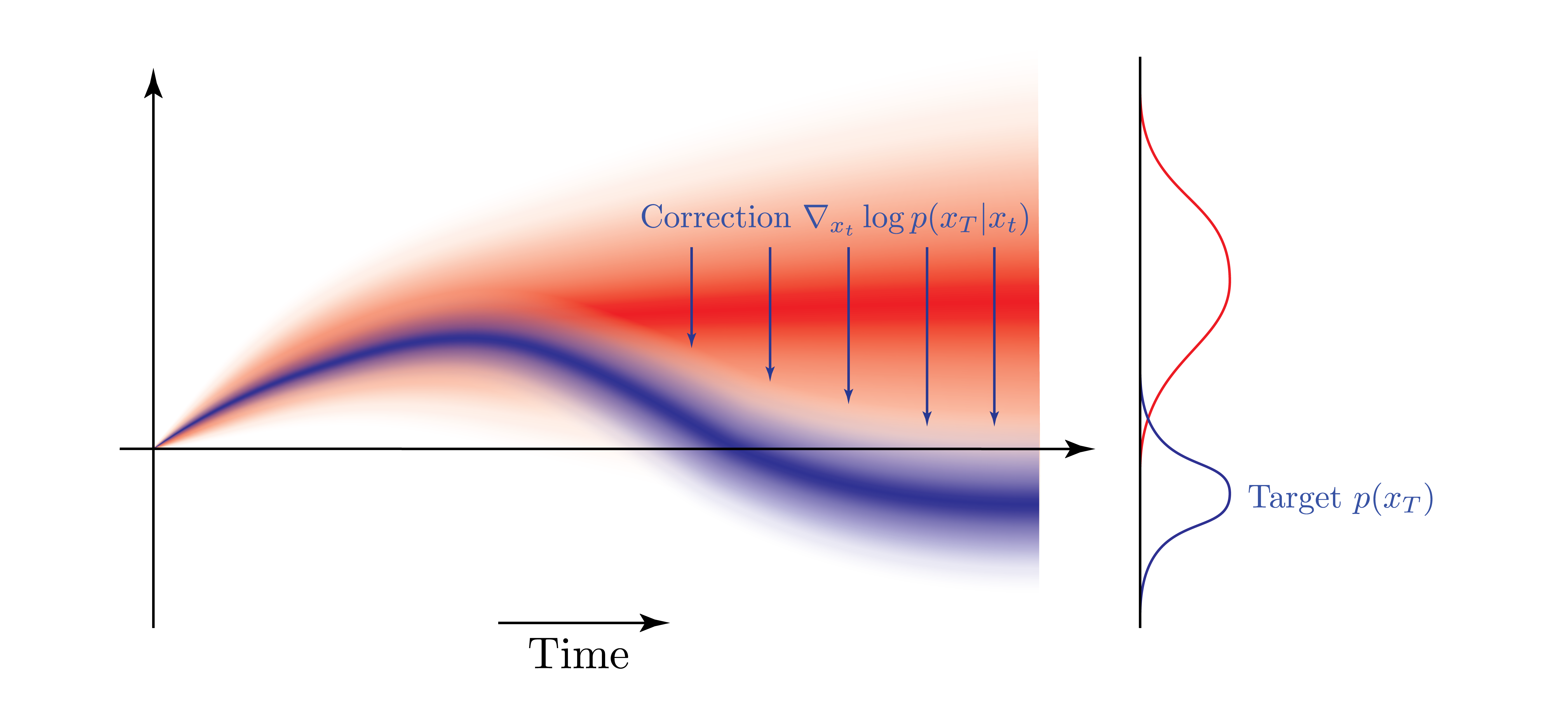
Doob's h-Transform

Previously, we saw how Girsanov’s theorem is little else than importance sampling for stochastic processes.

This time I stumbled over Doob’s h-transform. On first reading is an equally strange equation which seemed hard to understand when simply googling for it. But peeling away the layers like an onion and almost crying an equal amount along the way, there was some simply and intuitive things to be found.

The Purpose

To get it core idea out of the way: Doob’s h-transform is a way to condition a stochastic process on a future event. The obvious question is how to achieve such a condition.

For that we first observe our favourite equation on this blog, a stochastic differential equation in the form of an Ito drift-diffusion process

Next, we want to posit the probability of a future state $x_T$ at the end of our stochastic process given our current state $x_t$, $p(x_T | x_t)$. The probability simply states how probable our terminal future state $x_T$ is, given our current state $x_t$. Just a plain conditional probability.

Instead of going all the way to $t=T$ we can equally go to $t+\Delta t$ and denote the same transition probability $p(x_{t+\Delta t} | x_t)$. We can then construct the Chapman-Kolmogorov equation to integrate out over the $x_{t+\Delta t}$ to obtain

which states little else than considering every path from $x_t$ to $x_{t+\Delta t}$ and subsequently from $x_{t+\Delta t}$ to $x_T$. If we consider every possible $x_{t+\Delta t}$ in between $x_t$ and $x_T$, we simply marginalize $x_{t+\Delta t}$ out.

Rewriting the Chapman-Kolmogorov equation above yields an interesting identity,

which is the definition of a martingale.

The martingale equation above tells us that the probability of hitting $x_T$ given $x_t$ is the same as doing a step with the transition kernel $p(x_{t+\Delta t} | x_t)$ and then computing the probability of hitting $x_T$ from state $x_{t+\Delta t}$. Said more succinctly, our “predictive” power of $p(x_T | x_t)$ stays the same, regardless of doing a step to $x_{t+\Delta t}$. Obviously this only holds in the expected sense and sure enough there can massive spikes when considering extreme paths. But on average, we gain precisely no new information.

The notation of the probability $p(x_T , T | x_t, t)$ is just a more instructive way of signalling what $x_t$ will be used for but is nevertheless still a function of just $x_t$. We can abstract a bit more and write the martingale in terms of a function $f(x_t)$,

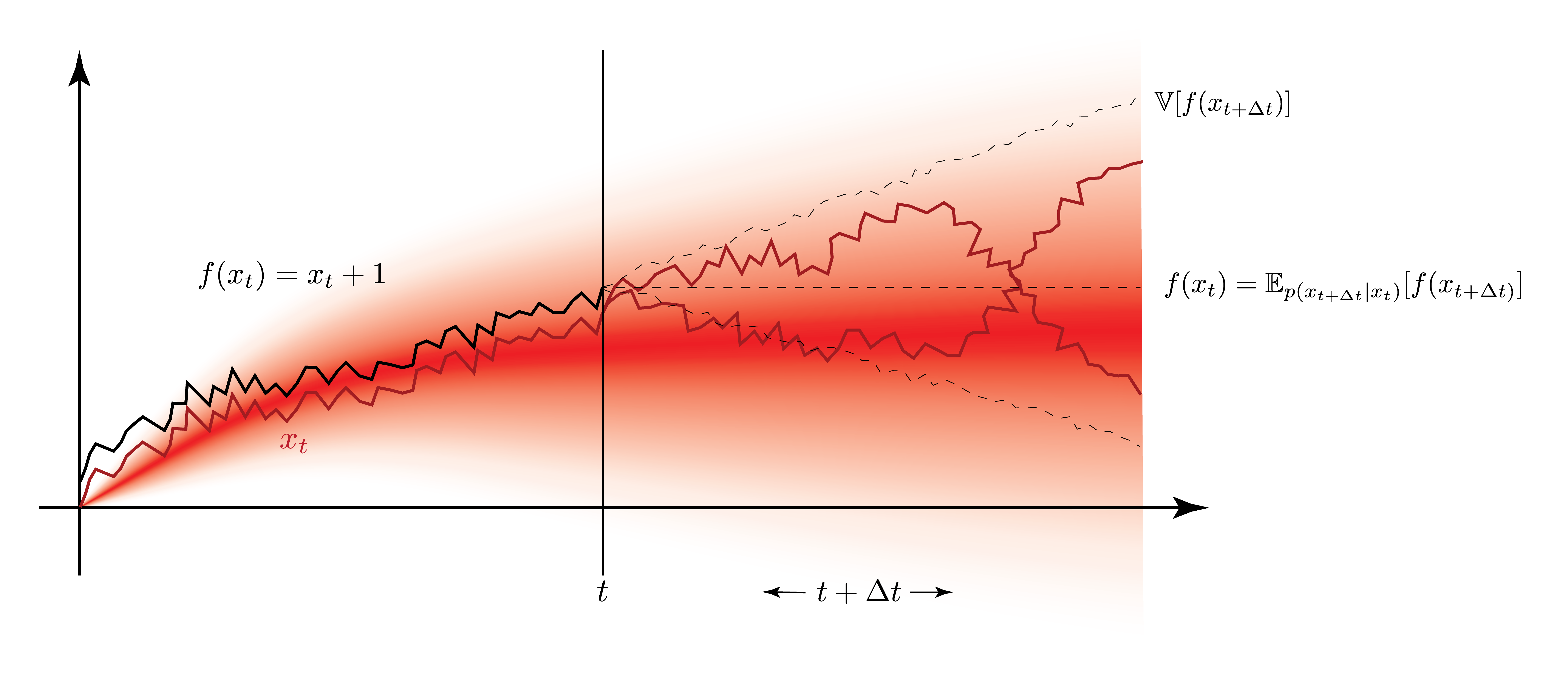
Below is a figurative representation of a Martingale. We use a simple function $f(x_t) = x_t + 1$ and if the drift of the SDE is zero, then we have a Martingale property. Thus from the moment on where we’re only dealing with a pure diffusive process with no drift, we will not be able to make an educated guess on what the future value of $f(x_{t+\Delta t})$ will be. Naturally, the variance can still increase, but on average, we can’t predict more than we know at $t$.

We will continue right after these commercials on the Kolmogorov Backward Equation… (insert advertisement jingle)

Commercial 1: The Kolmogorov Backward Equation

So how exactly does $p(x_T | x_t)$ change if we change $x_t$? What are the dynamics of $p(x_T | x_t)$? The probability $p(x_T | x_t)$ is little else than a function that takes in $x_t$ and outputs a scalar value. We further know that the change in $x_t$ is driven by the stochastic differential equation above. So, it’s time to use Ito’s lemma once again! But first we’ll make the following derivation more general by abbreviating $p(x_T, T | x_t, t) = f(x_t, t)$.

What happens if $\Delta t$ goes to zero?

With Ito’s lemma we know how to apply a Taylor expansion to a function the input of which is governed by a SDE. Applying Ito’s lemma to the term in the expectation we obtain

All the terms in the expectation are deterministic except the Brownian motion $dW_t$. Fortunately, we know that the expectation $\mathbb{E} [ dW_t]=0$, as this is one of the core properties of Brownian motion. Thus the equation above reduces after applying the expectation to

Cancelling the $f(x_t, t)$ and dividing zero by $dt$ on both sides gives us the Kolmogorov backward equation,

One of our assumptions is that $x_T$ remains fixed during all our mathematical shenanigans and thus we can plug back in our distribution $p(x_T, T | x_t, t)=f(x_t, t)$ where all the partial derivatives apply to the $x_t$ and $t$ components, not the $x_T$ and $T$!

Thus we obtain

where again $p(x_T,T|x_t,t)$ is purely a function of $x_t$ (as in $f(x_t, t)$) and is notationally written more elaborately as $p(x_T,T |x_t,t)$.

Commercial 2: Kolmogorov Forward solves a different problem than the Kolmogorov Backward

I personally asked myself why the derivation of the Kolmogorov Forward (aka Fokker-Planck) was different from the Kolmogorov Backward Equation.

At it’s core, the backward equation focuses on the evolution of expectations of functions of the process, conditioning on the current state while evolving backward in time. It addresses how a future payoff (or terminal condition) depends on the present state when viewed from the future time.

The forward equation focuses on the time evolution of the distribution, describing how probabilities evolve forward from an initial condition. Naturally you can integrate the FPE PDE also backwards in time. While their name might be direct opposites, the KBE and KFE solve wholly different problems. The resulting forward and backward equations have very similar structure, only differing in terms of the signs and how the derivatives are applied. Whereas the FPE/KFE models the interaction between the drift, diffusion and the resulting marginal probability distribution, the KBE only a evaluates a function which never interferes with the dynamics.

Commercial 3: The Infinitisimal Generator

Let us consider again the Martingale property

Pulling $f(x_t, t)$ to the right side we get

Since mathematicians are lazy by nature (and it’s significantly more convenient down the road), we abbreviate the term in the curly braces as $\mathcal{A}_t \ f$. In this notation, the SDE drift $\mu(x_t, t)$ and diffusion $\sigma(x_t, t)$ is absorbed into the operator $\mathcal{A}_t$. The equation above states that the difference between the current value $f(x_t, t)$ and the expected future value is equal to the operator $\mathcal{A}_t$ applied to the function itself and scaled with the time difference.

All that is left to do is to pull the $dt$ via a division to the other side and take the limit $\lim {dt \rightarrow 0^+}$ .

We get

The three terms above say the following: The expected, infinitisimal change of a function, the input of which is driven by a SDE, can be written as partial differential equation. The operator $\mathcal{A}_t$ encapsulates all relevant SDE terms and partial derivatives into a single operator.

Commercial Break is Over

With a bit of foresight, we will define a new transition kernel $\tilde{p}(x_{t+\Delta t} | x_t)$ for a slightly adjusted Markov process such that our target value of $p(x_T | x_t)$ is included in the transition kernel,

Before, we had defined the transition kernel $p(x_{t+\Delta t} | x_t)$ which is, based on the SDE being Markovian, also Markovian. The SDE above only takes the current state and nothing else to ‘predict’ the next state.

For $\tilde{p}(x_{t+\Delta t} | x_t)$ to be a proper Markovian transition kernel we have to show that $\int \tilde{p}(x_{t+\Delta t} | x_t) dx_{t+\Delta t} = 1$. We can show that via the Martingale property by simply integrating both sides and obtaining

With that proven, we can now define an infinitissimal generator under the transition kernel $\tilde{p}$. This is a kind expected finite difference between a state $x_t$ and a next state $x_{t+\Delta t}$ where we take the expected value over the slightly modified transition kernel $\tilde{p}$. We have

The term above shows that the infinitisimal generator $\mathcal{A}_t$ applied under the transition kernel $\tilde{p}$ is in fact a slightly modified infinitisimal generator itself.

Intriguing …

So let’s unpack the operator $\mathcal{A}_t$ and see what it’s hiding beneath. In a sense, all we have to do is to apply the differential operators included in $\mathcal{A}_t$ to the product of the two functions $f(x_t, t) p(x_T, T| x_t, t)$. In order to alleviate the notational burden, we will denote $f(x_t, t)$ without it’s arguments and abbreviate $p(x_T, T | x_t, t)$ by $h$.

So far, we’ve only differentiates once the functions $f: \mathbb{R}^N \rightarrow \mathbb{R}$ and $p: \mathbb{R}^N \rightarrow \mathbb{R}$ with $x \in \mathbb{R}^N$. Differentiating these functions once gives us vectors. But differentiating a second time, as will do with $\partial^2_{x_t} [f h]$ will differentiate the vector with respect to the vector valued input. Therefore, we have to pay special attention to the order of the differentiation in the sense of

Now, let’s put all these components back together again

where we observe that the terms highlighted in blue evaluate precisely to $0$ according to the Kolmogorov backward equation,

This simplifies our equation to

Remember how the Kolmogorov backward equation derived for a standard Ito SDE $dx_t = \mu(x_t, t) dt \sigma(x_t, t) dW_t$? We can go in reverse and read off a corresponding SDE that fulfills the particular Kolmogorov backward equation above,

Interestingly, this looks extremely similar to reverse-time diffusion as it’s used in diffusion based generative modelling in machine learning.