Black-Scholes Equation for Options Pricing

\(\newcommand{\Efunc}[1]{\mathbb{E}\left[ #1\right]} \newcommand{\Vfunc}[1]{\mathbb{V}\left[ #1\right]} \newcommand{\KL}[2]{\text{KL}\left[ #1 \ || \ #2 \right]} \newcommand{\denom}[1]{\frac{1}{#1}} \newcommand{\drift}{\mu(X_t, t)} \newcommand{\diff}{\sigma(X_t, t)}\)

The Black-Scholes equation is heralded as one rather important equations in finance, as it allows putting a precise price on an option within the Black-Scholes framework. It’s from economics, so as usual everything is assumed to be Gaussian distributed, statistically independent and linear. ;-)

But first, let’s try to frame the problem we’re dealing with properly. Namely,

• What is an Option?
• Why are they of relevance?
• Can we put a price tag on them like in Aldi?

The Option

An option in finance is a type of derivative contract that gives the buyer the right, but not the obligation, to buy or sell an underlying asset or instrument at a specified strike price prior to or on a specified date, depending on the form of the option. Derivatives in general are financial products which derive their value from another, usual more basic financial product. For example, you could take a kilo of gold and construct a derivative on the price of gold or the volatility of gold or inverse correlation to some interest rate or the correlation to another financial product. Since there is no limit to the creativity how exactly your derivative contract derives its value from the underlying asset, it’s no wonder that Warren Buffet called them ‘financial weapons of mass destruction’. Derivatives on housing prices in 2008 come to mind. Options are widely used for various purposes, including hedging, speculation, and acquiring or disposing of assets at favorable prices. They can apply to numerous assets, like stocks, bonds, commodities, and currencies.

There are two main types of options:

• Call Options: Grant the holder the right to buy the underlying asset at the strike price within a specified period. Investors buy call options if they anticipate an increase in the asset’s price.
• Put Options: Grant the holder the right to sell the underlying asset at the strike price within a specified period. Investors buy put options if they anticipate a decrease in the asset’s price.

The three important features of an option are:

• Premium: The price the option buyer pays to the seller for the rights granted by the option. After all you’re locking in preferential treatment at a later point in time.
• Strike Price: The predetermined price at which the option buyer can buy (call) or sell (put) the underlying asset.
• Expiration Date: The date by which the option must be exercised or it expires worthless.

The Relevance of Options

So let’s assume that a stock $S$ is worth $ \$ 100 $.

Further assume that for the time being we price a call option at $ \$ 10 $ in one years time. Thus if the stock rises above $ \$110 $, let’s say $ \$ 125$, we will make a profit of $ \$ 15 $ as we can buy the stock for $ \$ 100$ and immediately sell it for the $\$ 125$ and after subtracting the price of $\$ 10$ of our option, we have a profit of $\$15$. Nice, free money. If the stock $S$ stays below $\$110$, let’s say $\$ 108$ dollars it doesn’t really make sense to buy the stock at all to quickly sell it again, as we would buy high and sell low which is exactly the opposite of making a profit. In that case we lost the $\$ 10$ we paid for the option in the beginning.

But was the price of $\$ 10$ actually the correct price of the option? Let’s establish the value of the option as $V(S, t)$ which depends on the price of the underlying stock (naturally) and the time index $t$ which usually measures the time until expiration of the option. Next, we define our portfolio as $\Pi=\$110$ which is everything you have, be it stocks or cold, hard cash.

We can assume that in a world of ever increasing stock prices (thanks, Fed) we want to buy a stock $S$ and protect it against loosing its value. We can achieve this by buying a put option to sell the stock $S$ in one years time for the $\$100$ dollars we bought it for. Therefore, if the stock crashes to $\$1$, we can still demand from the seller of the put option to buy the stock for the full $\$100$ dollars and make us whole. For this peace of mind, we pay the seller of the put option the initial $\$ 10$.

But the option itself has a value as well as they are tradeable and can be sold and bought on specialized markets. Let a third person own the same stock and suddenly the stock crashes to $\$1$. If the third person could get to own our option, he could buy our option for its value $V(S, t)$ and force the seller of the option to buy his basically worthless stock for the full $\$100$. Thus it works as a sort of insurance to hedge a portfolio against sudden movements. The nice things about options is that we can sell respectively buy the stock for a predetermined price, but we don’t have to. That is how we can hedge our portfolio, and the overarching framework is called dynamic hedging. The dynamic part comes from us constantly selling and buying stocks $S$ and their options $V(S, t)$ in our portfolio $\Pi$ based on the behavior of the stock and our options.

We will now introduce the term $\Delta = \partial_S V(S, t)$ to express the sensitivity of the worth of the option with regards to changes in the price of the underlying stock $S$.

For a put option, this sensitivity is negative, $\Delta < 0$, since if the value of the stock $S$ is very low for an option with a high strike price, the put option itself becomes very valuable as it allows you to sell the worthless stock for the full agreed-upon price of $\$100$. So $V(S, t)$ and $S$ are negatively linked with $\Delta < 0$ as any drop in $S$ increases $V(S, t)$.

This allows us to offset the stock position $S$ in our portoflio $\Pi$ with put options $V(S, t)$ against possible drops in the value of the stocks! Namely, we have a hedged portfolio \(\begin{align} \Pi &= V(S, t) - \Delta S \\ &= V(S, t) - \partial_S V(S, t) \cdot S \end{align}\)

Let’s exemplify the behavior of $\Pi$.

We have bought the stock $S$ for $\$100$ and hedged it with a put option $V(S, t)$ to be able to sell it in one years time for the same $\$100$. Empirically, for put options for which the price of the underlying stock has dropped significantly from the strike price (the option is deep in the money), we can assume a $\Delta=-1$. Now a year has passed and the price of the stock $S$ is at a paltry $\$1$. The value of the option is the difference of the buy price of the underlying stock $S=\$1$ and the strike price of $\$100$ such that $V(S, t) = \$99$, which is the maximum profit you can make in this constellation of stock price and option value. In cases where owning an option provides a significant advantage, for example the stock is very low for a put option with high strike price or the stock price is very high for a call option with low strike price, an option is called ‘in the money’.

Since $S= \$1$ and $\Delta=-1$, we have \(\begin{align} \Pi &= V(S, t) - \partial_S V(S, t) \cdot S \\ &= \$99 - (-1) \cdot \$ 1 \\ &= \$ 100 \end{align}\) and we see that our portfolio as a whole has not budged from the initial $\$100$ dollars (we omitted the option premium and transaction costs and the like to strengthen the intuition).

Through the sensitivity of $\Delta = \partial_S V(S, t)$ we can construct a portfolio which is risk neutral. Come hell or high water in the financial markets, by properly adapting the ratio of stocks and options in your portfolio you can whether the storm and keep your money. Of course, this approach relies on an accurate estimation of the relevant sensitivity $\Delta$. This approach is named delta hedging after its main ingredient, $\Delta = \partial_S V(S, t)$.

Bob, the financier: Can we price $V(S, t)$? Yes we can! … with stochastic calculus

Naturally, the value of the option and consequently the portfolio $\Pi$ is driven by the behavior of the underlying stock $S$. The question thus arises of how exactly the price of the stock influences the price of the option and thus the portfolio itself. Therefore we are interested in the change in the portfolio \(\begin{align} d\Pi = dV(S, t) - \Delta \cdot dS \end{align}\) which is a differential equation which in turn is ‘driven’ by the differential $dV(S, t)$ and $dS$. Importantly, the portfolio makes only sense to maintain if equals a return rate on the safest instruments, US treasury bonds. If you’re making less with the fancy modelling than the US treasury bonds, this whole idea is not even worth pursuing. A useful and truly hedged portfolio needs to return the same amount, as if we were to invest all the cash in $\Pi$ into Uncle Sams bonds. Thus we have the following requirement \(\begin{align} d\Pi = r \Pi dt \end{align}\) which is the compounding interest of the whole portfolio invested with US treasury bonds.

One assumption of Black-Scholes model is that the stock price follows a geometric Brownian motion \(\begin{align} dS_t = \mu S dt + \sigma S dW_t \end{align}\) such that large stock prices incur larger movements in both drift and diffusion.

We are now interested in the dynamics of $dV(S, t)$ which hinges on the behavior of $S$ caputred by the SDE above.

Ito’s Lemma, derived and explained in more detail here and used for the derivation of the FPE here, gives us a straight forward equation for this: \(\begin{align} dV(S, t) = \left(\partial_t V(S, t) + \mu S \partial_S V(S, t) + \frac{1}{2} \sigma^2 S^2 \partial^2_S V(S, t) \right) dt + \sigma S \partial_S V(S, t) dW_t. \end{align}\)

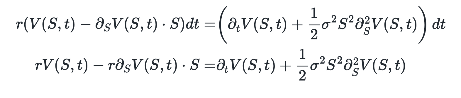
Now, we can plug in both the terms of $dV(S, t)$ and $dS$ to obtain \(\begin{align} d\Pi = & \left(\partial_t V(S, t) + \mu S \partial_S V(S, t) + \frac{1}{2} \sigma^2 S^2 \partial^2_S V(S, t) \right) dt + \sigma S \partial_S V(S, t) dW_t \\ & - \Delta \cdot \left( \mu S dt + \sigma S dW_t\right) \\ = & \left(\partial_t V(S, t) + \mu S \partial_S V(S, t) + \frac{1}{2} \sigma^2 S^2 \partial^2_S V(S, t) \right) dt + \sigma S \partial_S V(S, t) dW_t \\ & - \partial_S V(S, t) \cdot \left( \mu S dt + \sigma S dW_t\right) \\ = & \left(\partial_t V(S, t) + \color{blue}{\mu S \partial_S V(S, t)} + \frac{1}{2} \sigma^2 S^2 \partial^2_S V(S, t) \right) dt + \color{red}{\sigma \partial_S V(S, t) dW_t} \\ & - \color{blue}{\partial_S V(S, t) \mu S dt} - \color{red}{\partial_S V(S, t)\sigma S dW_t} \\ = & \left(\partial_t V(S, t) + \frac{1}{2} \sigma^2 S^2 \partial^2_S V(S, t) \right) dt \end{align}\) which is particularly interested as there is no diffusion term which indicates absolut deterministic dynamics as far as the portfolio dynamics are concerned. Since we equated the portfolio dynamics at a minimum to the risk free returns of government bonds, we equate another time to obtain \(\begin{align} r ( V(S, t) - \partial_S V(S, t) \cdot S) dt = & \left(\partial_t V(S, t) + \frac{1}{2} \sigma^2 S^2 \partial^2_S V(S, t) \right) dt \\ r V(S, t) - r \partial_S V(S, t) \cdot S = & \partial_t V(S, t) + \frac{1}{2} \sigma^2 S^2 \partial^2_S V(S, t) \end{align}\)

Thus, if we find a function $V(S, t)$ which for any value of $S$ and at any time $t$ fulfills the partial differential equation above, we will have a portfolio that generates at a minimum the risk free return and is hedged at all times. Consequentially, this also tells us the price of the specific option $V(S, t)$ given a specific stock price $S$.