Basics with Matrices
Back to University Math 101
Enter the Matrix
A matrix is little else than plain linear scaling but written in the most space and time saving way.
Take the equation \(y = a \cdot x\) which scales a number $x$ by a factor of $a$. What happens if we have multiple numbers and want to scale them all at once? For that we introduce little subscripts to indicate the first $x$ as $x_1$ and the second $x$ as $x_2$. Similarly, we denote the corresponding outputs as $y_1$ and $y_2$ and the scaling turning $x_1$ into $y_1$ as $a_1$ and the scaling turning $x_2$ into $y_2$ as $a_2$. So for example we would have $y_1 = a_1 \cdot x_1$ and $y_2 = a_2 \cdot x_2$ and so on. Stacking the $y_1$ and $y_2$ equations, we can it out as
\[\begin{align*} y_1 = a_1 \cdot x_1 \\ y_2 = a_2 \cdot x_2 \end{align*}\]In the equations above we’re clearly using $x_i$ as a single input to obtain a corresponding output $y_i$. Since Indian mathematicians came up with the concept of $0$ a long time ago, we can also theoretically add all the $x_i$’s to both equations by properly multiplying them by zero:
\[\begin{align*} y_1 = a_1 \cdot x_1 + 0 \cdot x_2 \\ y_2 = 0 \cdot x_1 + a_2 \cdot x_2 \end{align*}\]But now we for each $y_i$ have an expression that involves all the $x_i$’s, not just a single one. If we now want to distinguish that a particular $a_i$ is the scaling we use to scale a particular $x_j$, we need a way to indicate both what input $x_i$ is scaled how for each output $y_i$. So we have to denote each $a$ by it’s input and output indices $a_{\text{output} \leftarrow {\text{input}}}$. So we get
\[\begin{align*} y_1 = a_{1 \leftarrow 1} \cdot x_1 + \overbrace{a_{1 \leftarrow 2}}^{=0} \cdot x_2 \\ y_2 = \underbrace{a_{2 \leftarrow 1}}_{=0} \cdot x_1 + a_{2 \leftarrow 2} \cdot x_2 \end{align*}\]Writing arrows is cumbersome, especially for larger matrices, which is why mathematicians prefer the compact notation and we simply write $a_{ij}$ instead of $a_{i \leftarrow j}$ how input $x_j$ affects output $y_i$. Since this is just a sum, we can also write it as such:
\[\begin{align} y_1 &= \sum_{j} a_{1j} \cdot x_j \\ y_2 &= \sum_{j} a_{2j} \cdot x_j \end{align}\]Mathematicians are a lazy bunch, sorry, efficient bunch and they quickly become bored at writing out all these little subscripts $_1$ and $_2$ all the time, so they thought hard about how to write the two equations in a more compact form. The $y$’s, $a$’s and $x$’s only differ in their subscripts so we should be able to collect all the $y$’s, $a$’s and $x$’s into some sort of bundle up object that represents all of them at once, which leads us to the concept of vectors and matrices.
Let’s first collect the $y$’s and $x$’s and introduce introduce a collective object $\mathbf{x} = ( x_1 , x_2)$ and $\mathbf{y} = ( y_1 , y_2)$. This is straight forward as both $\mathbf{x}$ and $\mathbf{y}$ only have one dimension which is denoted by its single subscript. The $a$’s form a two-dimensional array since they have two subscripts which we call a matrix, and we denote it by
\(\mathbf{A} = \begin{bmatrix} a_{11} & a_{12} \\ a_{21} & a_{22} \end{bmatrix}\).
This brings us to the workhorse of linear algebra, the matrix-vector multiplication:
\[\begin{align*} \mathbf{y} &= \mathbf{A} \mathbf{x} \\ \begin{bmatrix} y_1 \\ y_2 \end{bmatrix} &= \begin{bmatrix} a_{11} & a_{12} \\ a_{21} & a_{22} \end{bmatrix} \begin{bmatrix} x_1 \\ x_2 \end{bmatrix} \\ &= \begin{bmatrix} a_{11} \cdot x_1 & + & a_{12} \cdot x_2 \\ a_{21} \cdot x_1 & + & a_{22} \cdot x_2 \end{bmatrix} \\ \end{align*}\]As a simple starting point, consider the diagonal matrix
\[\mathbf{A} = \begin{bmatrix} a_{11} & 0 \\ 0 & a_{22} \end{bmatrix}.\]But wait a second, if we squint really closely, we can rediscover the stacking we did with the vector $\mathbf{x}$ and $\mathbf{y}$ in the matrix $\mathbf{A}$ by interpreting the columns of the matrix as vectors as well:
\[\mathbf{A} = \begin{bmatrix} a_{11} & 0 \\ 0 & a_{22} \end{bmatrix} = \begin{bmatrix} \begin{bmatrix} a_{11} \\ 0 \end{bmatrix} & \begin{bmatrix} 0 \\ a_{22} \end{bmatrix} \end{bmatrix}.\]so our matrix $\mathbf{A}$ can be seen as a collection of vectors as well!
With this representation of a matrix, we can now reinterpret matrix-vector multiplication as a combination of the matrix’s column vectors:
\[\begin{align*} \mathbf{y} &= \mathbf{A} \mathbf{x} \\ \begin{bmatrix} y_1 \\ y_2 \end{bmatrix} &= \begin{bmatrix} \begin{bmatrix} a_{11} \\ a_{21} \end{bmatrix} & \begin{bmatrix} a_{12} \\ a_{22} \end{bmatrix} \end{bmatrix} \begin{bmatrix} x_1 \\ x_2 \end{bmatrix} \\ &= \begin{bmatrix} \begin{bmatrix} a_{11} \\ a_{21} \end{bmatrix} x_1 + \begin{bmatrix} a_{12} \\ a_{22} \end{bmatrix} x_2 \end{bmatrix} \\ &= \begin{bmatrix} a_{11} \\ a_{21} \end{bmatrix} x_1 + \begin{bmatrix} a_{12} \\ a_{22} \end{bmatrix} x_2 \end{align*}\]This now opens up a new interpretation as we’ve initially considered $\mathbf{y} = \mathbf{Ax}$ as the scaling of the input $\mathbf{x}$ by their respective $a$ coefficients. Now, we can also see it as forming the output $\mathbf{y}$ by combining the column vectors of $\mathbf{A}$, each scaled by the corresponding component of $\mathbf{x}$. Initially we thought about scaling $x$ with $a$, but now we’re flipping the script and scaling the column vectors in the matrix $\mathbf{A}$ by the components of $\mathbf{x}$.
The animation below highlights both of these approaches: We either interpret it as a scaling of the input $x$ by the values in $A$ through its column space. Alternatively, we interpret the linear transformation as a combination of the column space of $A$ through $x$.
Scaling a matrix-vector product
Vary A · fixed x
Fixed A · vary x
The column space view shifts the analysis from the input $x$ onto the matrix $A$ itself, opening up some interesting options which we will see below. We thus turn the matrix $\mathbf A$ from a simple object of writing scaling $x$ compactly into a first class citizen that warrants its own analysis tools and distinct properties. One of those analysis tools is the rank of a matrix.
Rank of a Matrix
When inspecting the column space of a matrix
\[\begin{align*} \mathbf{y} &= \mathbf{A} \mathbf{x} \\ \begin{bmatrix} y_1 \\ y_2 \end{bmatrix} &= \begin{bmatrix} \begin{bmatrix} a_{11} \\ a_{21} \end{bmatrix} & \begin{bmatrix} a_{12} \\ a_{22} \end{bmatrix} \end{bmatrix} \begin{bmatrix} x_1 \\ x_2 \end{bmatrix} \\ &= \begin{bmatrix} \begin{bmatrix} a_{11} \\ a_{21} \end{bmatrix} x_1 + \begin{bmatrix} a_{12} \\ a_{22} \end{bmatrix} x_2 \end{bmatrix} \\ &= \begin{bmatrix} a_{11} \\ a_{21} \end{bmatrix} x_1 + \begin{bmatrix} a_{12} \\ a_{22} \end{bmatrix} x_2 \end{align*}\]we can see that the resulting vector $\mathbf{y}$ is a linear combination of the columns of $\mathbf{A}$. Why? Because we’ve shifted from interpreting $a_{ij}$ as the linear coefficients to interpreting $x_i$ as the coefficient which scales the vectors in the column space of the matrix.
Consequently, we can ask what kind of vectors $\mathbf{y}$ we can generate from $\mathbf{A}$ for a given $x$. The answer to that is closely related to the rank of a matrix Let’s consider the matrix
\[A = \begin{bmatrix} \begin{bmatrix} 2.5 \\ 0 \end{bmatrix} & \begin{bmatrix} 0 \\ 0.5 \end{bmatrix} \end{bmatrix}\]which coincidentally can be interpreted as the basis vectors of a two dimensional coordinate system. A vector $\mathbf{x} = (x_1, x_2)$ scales the first column by $x_1$ and the second column by $x_2$
\[\begin{bmatrix} y_1 \\ y_2 \end{bmatrix} = \begin{bmatrix} 2.5 \\ 0 \end{bmatrix} x_1 + \begin{bmatrix} 0 \\ 0.5 \end{bmatrix} x_2\]The column space of $\mathbf{A}$ consists of two different vectors as they both point into different directions. Essentially both vectors stay out of each other’s lanes and don’t interfere across dimension with each other. But what happens if we flip the entries in the second column of $\mathbf{A}$?
\[\begin{bmatrix} y_1 \\ y_2 \end{bmatrix} = \begin{bmatrix} 2.5 \\ 0 \end{bmatrix} x_1 + \begin{bmatrix} 0.5 \\ 0 \end{bmatrix} x_2\]In this case regardless of what we use as input $\mathbf{x}$, the second dimension of our output vector $y_2$ will always be zero. This collapses the second dimension and in effect we can only generate a variable output in the first dimension. The important test is whether we have independent columns in the matrix $\mathbf{A}$ or whether the column space consists of collinear vectors. Collinear vectors simply mean that they all point into the same direction but can have different lengths.
To make it more interesting (as in not squashing things to zero) we can purposefully construct a column space where $\mathbf{a}_2$ is a multiple of $\mathbf{a}_1$, namely $\mathbf{a}_2=1/5 \cdot \mathbf{a}_1$.
\[\begin{align*} \begin{bmatrix} y_1 \\ y_2 \end{bmatrix} = \underbrace{\begin{bmatrix} 2.5 \\ 1 \end{bmatrix}}_{\mathbf a_1}x_1 + \underbrace{\begin{bmatrix} 0.5 \\ 0.2 \end{bmatrix}}_{\mathbf a_2} x_2. \end{align*}\]Both columns have two nonzero components, but the second remains a multiple of the first. From the column space view of a matrix, we’re essentially creating an output vector $\mathbf{y}$ as a linear combination of vectors that all point into the same direction. They therefore provide only one independent direction, and every output remains on the line to which the columns point, just with possibly different lengths. We say that the matrix $\mathbf{A}$ has rank 1 even if it has more than 1 vectors in its column space, as it provides only one independent direction in its column space.
In the widget below, you can see that we can move the output vector $\mathbf{y}$ by adjusting the components of the input vector $\mathbf{x}$. In the $\text{rank}[A]=1$ case on the right, the output vector $\mathbf{y}$ is constrained to move along a single line, reflecting the fact that the column space of $\mathbf{A}$ has only one independent direction. If all vectors which we scale with $x_i$ point in the same direction, we’re strictly constrained to the subspace that are spanned by those collinear vectors as our basis system doesn’t allow for anything else.
Two independent directions, or one?
Independent columns
rank(A) = 2Outputs fill an area.
Collinear columns
rank(A) = 1Outputs stay on a line.
Both panels use this x. Shading shows outputs for −2 ≤ x₁, x₂ ≤ 2.
Matrix Inverse
The rank discussion gives us a natural way to understand why some matrices have an inverse and others do not. The rank-one transformation can be viewed as a many-to-one map. So far we’ve covered how we can compute $\mathbf y = \mathbf A \mathbf x$ given some input $\mathbf x$. But now we might be interested to obtain the $\mathbf x$ that created $\mathbf y$ in the first place. So the natural thing to ask is “What is the inverse matrix $\mathbf A^{-1}$ with which we can compute $\mathbf x = \mathbf A^{-1} \mathbf y$?”. Is there anything we should pay attention to in the properties of the matrix $\mathbf A$ before we tackle this idea?
Recall our rank-one matrix
\[\mathbf{A} = \begin{bmatrix} 2.5 & 0.5 \\ 1 & 0.2 \end{bmatrix},\]whose second column is a multiple of its first. Its matrix-vector multiplication can be written as
\[\begin{align*} \mathbf{A}\mathbf{x} &= \begin{bmatrix} 2.5 \\ 1 \end{bmatrix}x_1 + \begin{bmatrix} 0.5 \\ 0.2 \end{bmatrix}x_2 \\ &= \begin{bmatrix} 2.5 \\ 1 \end{bmatrix}x_1 + \frac{1}{5}\begin{bmatrix} 2.5 \\ 1 \end{bmatrix}x_2 \\ &= \begin{bmatrix} 2.5 \\ 1 \end{bmatrix} \underbrace{\left(x_1+\frac{1}{5}x_2\right)}_{\in \mathbb{R}}. \end{align*}\]Although we multiplied a two-dimensional input, $x_1$ and $x_2$, into the matrix, the output is determined by the direction of the column space of the matrix scaled by a linear combination of the input components. Whatever two values $x_1$ and $x_2$ we choose, the direction of the resulting output vector $\mathbf{y}$ remains the same and the input only appears for determining the length of the vector. The entire two-dimensional input plane is squashed onto the one-dimensional line spanned by the vector $\begin{bmatrix}2.5 & 1\end{bmatrix}^{\mathsf T}$. Said differently, the $x_1 + \frac{1}{5}x_2$ is a scaling factor but which does not affect the direction of $\begin{bmatrix}2.5 & 1\end{bmatrix}^{\mathsf T}$ but only its length. The problem is many different inputs can lead to the same output, making it impossible to uniquely determine the original input from the output alone. In other words, the matrix $\mathbf{A}$ has lost information about the input $\mathbf{x}$ that cannot be recovered from the output.
This creates a kind of mathematical trapdoor: many different inputs fall onto the same output. For example, consider the two inputs
\[\mathbf{x}^{(1)} = \begin{bmatrix} 1 \\ 0 \end{bmatrix}, \qquad \mathbf{x}^{(2)} = \begin{bmatrix} 0 \\ 5 \end{bmatrix}.\]They are clearly different, but both produce exactly the same output:
\[\mathbf{A}\mathbf{x}^{(1)} = \begin{bmatrix} 2.5 \\ 1 \end{bmatrix} (1 + \frac{1}{5} \cdot 0) = \begin{bmatrix} 2.5 \\ 1 \end{bmatrix} = \begin{bmatrix} 2.5 \\ 1 \end{bmatrix} (0 + \frac{1}{5} \cdot 5) = \mathbf{A}\mathbf{x}^{(2)}\]Now imagine that we are only given the output $\mathbf{y}=(2.5, 1)$ and are asked to recover the input. Was the input $\mathbf{x}^{(1)}$, $\mathbf{x}^{(2)}$, or one of infinitely many other possibilities? The matrix has discarded the information required to choose a unique answer for $\mathbf x$.
We can see the lost information by subtracting the two inputs to obtain the null space of the matrix $\mathbf{A}$. The null space are all the vectors which get mapped to the zero vector by the matrix.
\[\mathbf{A} \left( \mathbf{x}^{(2)}-\mathbf{x}^{(1)} \right) = \begin{bmatrix} 2.5 & 0.5 \\ 1 & 0.2 \end{bmatrix} \begin{bmatrix} -1 \\ 5 \end{bmatrix} = \begin{bmatrix} 0 \\ 0 \end{bmatrix}.\]The direction $(-1, 5)$ belongs to the null space of $\mathbf{A}$. Moving the input in this direction does not move the output at all:
\[\mathbf{A} \left( \mathbf{x} +t\begin{bmatrix}-1 \\ 5\end{bmatrix} \right) = \mathbf{A} x + t \underbrace{\mathbf{A} \begin{bmatrix}-1 \\ 5\end{bmatrix}}_{=\mathbf{0}} = \mathbf{A}\mathbf{x}\]for any value of $t$. All inputs along this line are indistinguishable after applying $\mathbf{A}$. So any vector $\mathbf{x}$ that is a scaled version of $(-1, 5)$ will be mapped to the zero vector by $\mathbf{A}$.
An inverse matrix is supposed to undo a matrix transformation. If
\[\mathbf{y}=\mathbf{A}\mathbf{x},\]then we would like to apply another matrix $\mathbf{A}^{-1}$ that recovers the original input. This is nothing else than the scalar case of $y =ax$ and getting $x = y / a$:
\[\mathbf{x}=\mathbf{A}^{-1}\mathbf{y}.\]Doing something and then undoing it should be equivalent to doing nothing, so an inverse must satisfy
\[\mathbf{A}^{-1}\mathbf{A} = \mathbf{A}\mathbf{A}^{-1} = \mathbf{I}.\]But our rank-one matrix cannot have such an inverse. If it did, applying $\mathbf{A}^{-1}$ to the collision above would give
\[\mathbf{x}^{(1)} = \mathbf{A}^{-1} y = \mathbf{A}^{-1}\mathbf{A} \underbrace{\mathbf{x}^{(1)}}_{=y} = \mathbf{A}^{-1} \underbrace{\mathbf{A}\mathbf{x}^{(2)}}_{=y} = \mathbf{x}^{(2)},\]even though the two inputs are different. This is again because multiple inputs $\mathbf{x}^{(1)}$ or $\mathbf{x}^{(2)}$ can be mapped to the same output $\mathbf{y}$ by a rank-deficient matrix.
Below is a little animation in which you can drag and move a vector $\mathbf{x}$ and see how it is mapped by the matrix $\mathbf{A}$ to it’s output $\mathbf{y}$. In the left animation, there is a line of inputs that all get mapped to the same output. Since all points on that line get mapped to the same point, we can not uniquely recreate the input vice-versa.
A rank-one matrix forgets one direction
Input space
Drag the first two points along the dashed line. Move the third freely.It is a shifted null space: A−1(y) = x(1) + ker(A).
Output space
The first two outputs coincide; the free point still lands on the same line.a2 = 0.2a1 · rank(A) = 1
This gives us the essential condition for invertibility:
A square matrix is invertible exactly when it has full rank.
Determinants of Matrices
The previous sections asked whether a matrix preserves all directions or squashes some of them together. The determinant packages the same geometric story into a single number: it tells us how a matrix scales area.
We begin with the simplest case, a diagonal matrix:
\[\begin{align*} \mathbf{A} &= \begin{bmatrix} a_{11} & 0 \\ 0 & a_{22} \end{bmatrix} = \underset{ \begin{array}{cc} \underbrace{\hphantom{\begin{bmatrix} a_{11} \\ 0 \end{bmatrix}}}_{\mathbf{a}_1} & \underbrace{\hphantom{\begin{bmatrix} 0 \\ a_{22} \end{bmatrix}}}_{\mathbf{a}_2} \end{array} }{ \begin{bmatrix} \begin{bmatrix} a_{11} \\ 0 \end{bmatrix} & \begin{bmatrix} 0 \\ a_{22} \end{bmatrix} \end{bmatrix} }. \end{align*}\]The first column stays on the horizontal axis and the second stays on the vertical axis. Consequently, the unit square becomes a rectangle with side lengths $\lvert a_{11}\rvert$ and $\lvert a_{22}\rvert$, and therefore with area $\lvert a_{11}\rvert\lvert a_{22}\rvert=\lvert a_{11}a_{22}\rvert$. The corresponding signed area is
\[\det(\mathbf{A})=\sqrt{a_{11}^2 + 0^2} \sqrt{0^2 + a_{22}^2} = \sqrt{a_{11}^2} \sqrt{a_{22}^2} = |a_{11}| |a_{22}|.\]Drag the two column vectors below. They are constrained to their respective axes, making it visible that each diagonal entry scales one side independently and that their product scales the area.
Now we let the columns point in arbitrary directions:
\[\begin{align*} \mathbf{A} &= \begin{bmatrix} a_{11} & a_{12} \\ a_{21} & a_{22} \end{bmatrix} = \begin{bmatrix} \begin{bmatrix} a_{11} \\ a_{21} \end{bmatrix} & \begin{bmatrix} a_{12} \\ a_{22} \end{bmatrix} \end{bmatrix}. \end{align*}\]The transformed unit square is still spanned by the two columns, but its right angles can now lean into a general parallelogram. Its signed area is
\[\det(\mathbf{A})=a_{11}a_{22}-a_{12}a_{21}.\]This is a deceptively simple equation which you will read in most text books. In order to understand how this simple subtractions comes to be, play around with the widget below which shows how we subtract the triangles from the parallelogram to obtain the term above. The determinant can be calculated by computing the outer bounding box and subtracting all triangles between the outer most bounding box and the actual parallelogram.
The magnitude $\lvert\det(\mathbf{A})\rvert$ is the area-scaling factor. A determinant of $2$ doubles every area, while a determinant of $1/2$ halves it. The sign keeps track of orientation: a positive determinant preserves the ordering of the two directions, while a negative determinant flips it, like turning a sheet of paper over.
This zero-area case is exactly the rank collapse from before. When the columns are collinear (try it out by making both vectors of the parallelogram identical in their direction), the matrix maps the plane onto a line, so $\det(\mathbf{A})=0$ and the lost direction makes the matrix non-invertible. When $\det(\mathbf{A})\neq 0$, the columns span the plane and the matrix is invertible. In higher dimensions the same idea remains: the determinant is the signed scaling factor for $n$-dimensional volume.
The determinant is associative in the sense if we want to know how a matrix $\mathbf{A}$ and a matrix $\mathbf{B}$ change a vector, we can chain the operations and compute each determinant separately, and then multiply them.
\[\det[AB] = \det[A] \det[B]\]This makes intuitively sense because applying two transformations in sequence should scale areas by the product of their individual scaling factors.
Trace of a Matrix
The trace of a square matrix is the sum of its diagonal entries:
\[\operatorname{Tr}(\mathbf{A}) = \sum_j a_{jj}.\]For a two-dimensional matrix, this is simply
\[\operatorname{Tr} \left( \begin{bmatrix} a_{11} & a_{12} \\ a_{21} & a_{22} \end{bmatrix} \right) = a_{11}+a_{22}.\]Recall that $a_{ij}$ describes how input component $x_j$ contributes to output component $y_i$. The diagonal entries are therefore the contributions that remain in the same coordinate: $a_{11}$ maps the first input direction back onto the first output direction, and $a_{22}$ does the same for the second. The off-diagonal entries mix one direction into another and do not contribute to the trace.
At first, adding the diagonal entries may appear arbitrary. Its geometric meaning becomes visible when we apply a very small transformation. Consider the matrix $\mathbf{I}+\delta\mathbf{A}$, where $\delta$ is a small number:
\[\mathbf{I}+\delta\mathbf{A} = \begin{bmatrix} 1 & 0 \\ 0 & 1 \end{bmatrix} + \delta \begin{bmatrix} a_{11} & a_{12} \\ a_{21} & a_{22} \end{bmatrix} = \begin{bmatrix} 1+\delta a_{11} & \delta a_{12} \\ \delta a_{21} & 1+\delta a_{22} \end{bmatrix}.\]The identity matrix leaves an area unchanged. The additional term $\delta\mathbf{A}$ applies a small deformation. To see how this deformation changes area, we calculate the determinant:
\[\begin{align*} \det(\mathbf{I}+\delta\mathbf{A}) &= (1+\delta a_{11})(1+\delta a_{22}) -\delta^2 a_{12}a_{21} \\ &= 1+\delta(a_{11}+a_{22}) +\delta^2(a_{11}a_{22}-a_{12}a_{21}). \end{align*}\]Because $\delta$ is small, $\delta^2$ is much smaller. If we focus only on the first-order change and ignore the $\delta^2$ term, we obtain
\[\det(\mathbf{I}+\delta\mathbf{A}) \approx 1+\delta(a_{11}+a_{22}) = 1+\delta\operatorname{Tr}(\mathbf{A}).\]The trace therefore measures the immediate rate at which a small transformation expands or contracts area. A positive trace means local expansion, a negative trace means local contraction, and a zero trace means that there is no first-order change in area.
The trace also has a useful cyclic property. Although matrix multiplication generally does not commute, the trace operator actually does $\operatorname{Tr}(\mathbf{B}\mathbf{C})=\operatorname{Tr}(\mathbf{C}\mathbf{B})$. Writing out the diagonal entries makes the reason visible:
\[\begin{align*} \operatorname{Tr}(\mathbf{B}\mathbf{C}) &= \sum_i(\mathbf{B}\mathbf{C})_{ii} = \sum_i\sum_j b_{ij}c_{ji} \\ &= \sum_j\sum_i c_{ji}b_{ij} = \sum_j(\mathbf{C}\mathbf{B})_{jj} \\ &= \operatorname{Tr}(\mathbf{C}\mathbf{B}). \end{align*}\]The entries $b_{ij}$ and $c_{ji}$ are ordinary numbers, so their multiplication commutes, and we can reorder the finite sums. The only thing we’ve really done is to switch the order of $c_{ji}$ and $b_{ji}$ while also switching out the sum operators. This does not mean that $\mathbf{B}\mathbf{C}=\mathbf{C}\mathbf{B}$, only that their traces agree. For three or more factors, this property allows us to rotate their order cyclically:
\[\operatorname{Tr}(\mathbf{B}\mathbf{C}\mathbf{D}) = \operatorname{Tr}(\mathbf{C}\mathbf{D}\mathbf{B}) = \operatorname{Tr}(\mathbf{D}\mathbf{B}\mathbf{C}).\]We cannot generally swap arbitrary factors, but we can move the first factor to the back.
The “Eigenheiten” of Matrices
What happens to individual directions under the transformation $\mathbf{A}$? Is there a nonzero vector whose direction survives without being turned, changing only in length or orientation?
Finding an eigenvector
Move the teal tip. Most directions turn under the transformation.
Drag the teal input tip. With the tip focused, use the arrow keys to move it, or hold Shift for larger steps. The input cannot be moved onto the zero vector.
Such a vector satisfies
\[\mathbf{A}\mathbf{v}=\lambda\mathbf{v} \quad \text{with } \mathbf{v} \neq \mathbf{0}\]We call $\mathbf{v}$ an eigenvector and $\lambda$ its eigenvalue. To be a bit on the nose: An eigenvector only changes its length via its corresponding eigenvalue and not its direction. Rearranging gives
\[(\mathbf{A}-\lambda\mathbf{I})\mathbf{v}=\mathbf{0}.\]Now remember our null space conversation: a vector lies in the null space of a matrix if and only if the matrix maps it to the zero vector. For a particular eigenvalue $\lambda$, the corresponding eigenvector $\mathbf{v}$ satisfies $(\mathbf{A}-\lambda\mathbf{I})\mathbf{v}=\mathbf{0}$.
Above we stated that the eigenvector $\mathbf{v}$ is nonzero. If it were nonzero, we would obtain the trivial solution $\mathbf{A} \mathbf{0}=\lambda\mathbf{0}$, which is a trivial eigenvector and more importantly would hold for any $\mathbf{A}$ and for any $\lambda$ at all times. So it’s kind of pointless, to be honest. A nontrivial null space means that some nonzero direction with arbitrary length is mapped to zero. Moving an input along this direction does not change its output:
\[(\mathbf A-\lambda\mathbf I)(\mathbf x+\mathbf v) = (\mathbf A-\lambda\mathbf I)\mathbf x + \underbrace{(\mathbf A-\lambda\mathbf I)\mathbf v}_{=0} = (\mathbf A-\lambda\mathbf I)\mathbf x.\]Different inputs along the direction of $\mathbf v$ therefore produce the same output, so no inverse can uniquely recover the original input. Hence, $\mathbf A-\lambda\mathbf I$ is not invertible. A non-invertible matrix has a determinant of zero, which gives us the characteristic equation for finding eigenvalues:
\[\det(\mathbf{A}-\lambda\mathbf{I})=0.\]For a two-dimensional matrix, we can write this equation out component by component:
\[\begin{align*} \det(\mathbf{A}-\lambda\mathbf{I}) &= \det\left( \begin{bmatrix} a_{11} & a_{12} \\ a_{21} & a_{22} \end{bmatrix} - \begin{bmatrix} \lambda & 0 \\ 0 & \lambda \end{bmatrix} \right) \\ &= \det\left( \begin{bmatrix} a_{11}-\lambda & a_{12} \\ a_{21} & a_{22}-\lambda \end{bmatrix} \right) \\ &= (a_{11}-\lambda)(a_{22}-\lambda)-a_{12}a_{21} \\ &= \lambda^2-(a_{11}+a_{22})\lambda +a_{11}a_{22}-a_{12}a_{21} =0. \end{align*}\]This equation allows us to find the eigenvalues. Once $\lambda$ is known, the corresponding eigenvectors are the nonzero vectors in $\ker(\mathbf{A}-\lambda\mathbf{I})$.
Geometrically, an eigenvector marks a line preserved by the transformation, while its eigenvalue tells us whether that line is stretched, compressed, flipped, or collapsed. These directions are the natural axes of the transformation.
Drag $\mathbf{x}$ below and hunt for a direction that the matrix does not turn.
We can make the relationship between eigenvectors and the column space precise using our rank-one matrix from before:
\[\mathbf{A} = \begin{bmatrix} 2.5 & 0.5 \\ 1 & 0.2 \end{bmatrix} = \begin{bmatrix} \mathbf{a}_1 & \mathbf{a}_2 \end{bmatrix}, \qquad \mathbf{a}_2=0.2\mathbf{a}_1, \qquad \mathbf{a}_1= \begin{bmatrix}2.5\\1\end{bmatrix}.\]Its characteristic equation is
\[\det(\mathbf{A}-\lambda\mathbf{I}) = (2.5-\lambda)(0.2-\lambda)-0.5 = \lambda(\lambda-2.7) =0,\]so the eigenvalues are $\lambda=2.7$ and $\lambda=0$. Substituting $\lambda=2.7$ into $(\mathbf{A}-\lambda\mathbf{I})\mathbf{v}=\mathbf{0}$ gives
\[\begin{bmatrix} -0.2 & 0.5 \\ 1 & -2.5 \end{bmatrix} \mathbf{v} = \begin{bmatrix} -0.2 v_1 & 0.5 v_2 \\ 1 v_1 & -2.5 v_2 \end{bmatrix} = \begin{bmatrix} 0 \\ 0 \end{bmatrix}.\]This is just a set of linear equations which we can solve to find the eigenvector $\mathbf{v} = [2.5 \; 1]^\mathsf{T}$ corresponding to $\lambda=2.7$. Substituting $\lambda=0$ similarly gives multiples of $\mathbf{v}=(-1,5)^\mathsf{T}$.
Decompositions of a Matrix
The eigenvector relationship actually gives us a neat entry into a matrix decomposition. We have the eigenvectors and eigenvalues relationship for each individual eigenvector, and by stacking them into matrices, we can express the entire decomposition compactly.
For a single eigenvector, we have
\[\mathbf{A}\mathbf{v}_i=\lambda_i\mathbf{v}_i.\]If $\mathbf{A}$ has enough linearly independent eigenvectors, we can stack them as the columns of a matrix
\[\mathbf{V} = \begin{bmatrix} \mathbf{v}_1 & \mathbf{v}_2 & \cdots & \mathbf{v}_n \end{bmatrix}.\]Each column of $\mathbf{V}$ interacts with the matrix $\mathbf{A}$ independently of the other eigenvectors. That’s just the property of a matrix matrix multiply. Conversely, on the right hand side with the eigenvalues $\lambda_i$, we have to scale each of the eigenvectors correspondingly by its eigenvalue:
\[\boldsymbol{\Lambda} = \begin{bmatrix} \lambda_1 & 0 & \cdots & 0 \\ 0 & \lambda_2 & \cdots & 0 \\ \vdots & \vdots & \ddots & \vdots \\ 0 & 0 & \cdots & \lambda_n \end{bmatrix}.\]Multiplying $\mathbf{V}$ by this diagonal matrix scales each column by its corresponding eigenvalue:
\[\mathbf{V}\boldsymbol{\Lambda} = \begin{bmatrix} \lambda_1\mathbf{v}_1 & \lambda_2\mathbf{v}_2 & \cdots & \lambda_n\mathbf{v}_n \end{bmatrix}.\]We have therefore bundled all the individual eigenvector equations into
\[\mathbf{A}\mathbf{V}=\mathbf{V}\boldsymbol{\Lambda}.\]Since we’re assuming a full rank matrix, the columns of $\mathbf{V}$ are linearly independent and $\mathbf{V}$ is invertible. Multiplying both sides from the right by $\mathbf{V}^{-1}$ gives
\[\mathbf{A} = \mathbf{V}\boldsymbol{\Lambda}\mathbf{V}^{-1}.\]This is the eigendecomposition. Read from right to left, $\mathbf{V}^{-1}$ changes into eigenvector coordinates, $\boldsymbol{\Lambda}$ scales each eigendirection independently, and $\mathbf{V}$ changes back. A matrix with enough independent eigenvectors for this construction is called diagonalizable.
The singular value decomposition extends the same intuition to every real matrix:
\[\mathbf{A}=\mathbf{U}\boldsymbol{\Sigma}\mathbf{V}^{\mathsf T}.\]Here, orthogonal changes of coordinates surround independent scalings. The number of nonzero singular values in $\boldsymbol{\Sigma}$ is exactly the rank of the matrix.
Matrix Exponentials
A matrix can describe not only one transformation, but also a transformation applied continuously. Consider the linear differential equation
\[\frac{d\mathbf{x}}{dt}=\mathbf{A}\mathbf{x}.\]Over a tiny interval $\Delta t$, the state changes approximately as
\[\mathbf{x}(t+\Delta t) \approx \left(\mathbf{I}+\Delta t\,\mathbf{A}\right)\mathbf{x}(t).\]Dividing a duration $t$ into $n$ tiny updates gives the matrix analogue of repeated scalar compounding:
\[\mathbf{x}(t) = \lim_{n\to\infty} \left(\mathbf{I}+\frac{t}{n}\mathbf{A}\right)^n \mathbf{x}(0) = e^{t\mathbf{A}}\mathbf{x}(0).\]Expanding this limit defines the matrix exponential:
\[e^{t\mathbf{A}} = \mathbf{I} +t\mathbf{A} +\frac{t^2\mathbf{A}^2}{2!} +\frac{t^3\mathbf{A}^3}{3!} +\cdots.\]Thus, $\mathbf{A}$ specifies the infinitesimal change, while $e^{t\mathbf{A}}$ accumulates it into the finite transformation after time $t$.
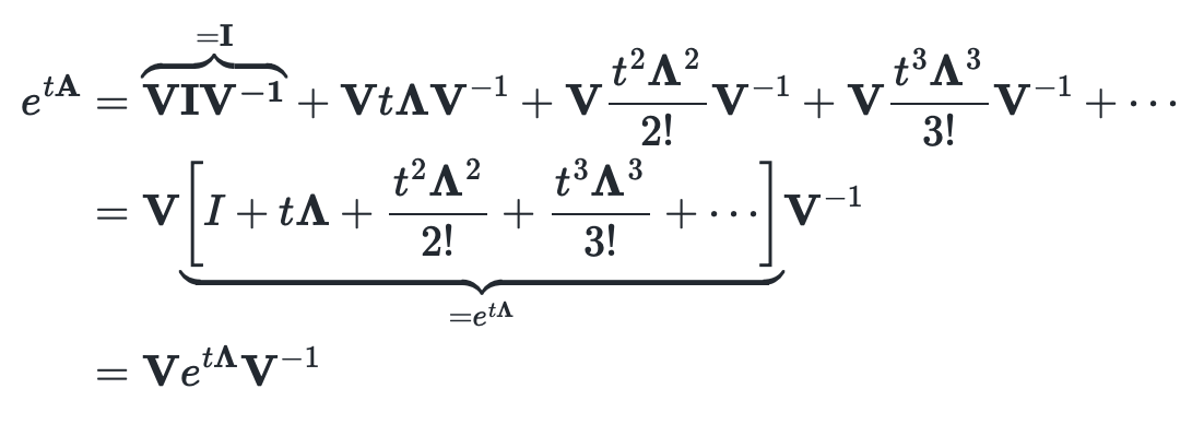
Previously we’ve encountered the eigendecomposition of a matrix in the form of $\mathbf{A}=\mathbf{V}\boldsymbol{\Lambda}\mathbf{V}^{-1}$. Let’s plug that eigendecomposition into the first three components that we have in the infinite sum of the matrix exponential:
\[\begin{align*} e^{t\mathbf{A}} &= \mathbf{I} +t\mathbf{A} +\frac{t^2\mathbf{A}^2}{2!} +\frac{t^3\mathbf{A}^3}{3!} +\cdots \\ &= \mathbf{I} +t\mathbf{A} +\frac{t^2\mathbf{A} \mathbf A}{2!} +\frac{t^3\mathbf{A} \mathbf{A} \mathbf{A}}{3!} +\cdots \\ &= \mathbf{I} +t\mathbf{V}\boldsymbol{\Lambda}\mathbf{V}^{-1} +\frac{t^2\mathbf{V}\boldsymbol{\Lambda}\mathbf{V}^{-1} \mathbf{V}\boldsymbol{\Lambda}\mathbf{V}^{-1}}{2!} +\frac{t^3\mathbf{V}\boldsymbol{\Lambda}\mathbf{V}^{-1} \mathbf{V}\boldsymbol{\Lambda}\mathbf{V}^{-1} \mathbf{V}\boldsymbol{\Lambda}\mathbf{V}^{-1}}{3!} +\cdots \\ \end{align*}\]Since $\mathbf V^{-1} \mathbf V = \mathbf I$ by definition of the inverse the intermediate terms between teh $\mathbf \Lambda$ disappear and we get
\[\begin{align*} e^{t\mathbf{A}} &= \mathbf{I} +t\mathbf{A} +\frac{t^2\mathbf{A}^2}{2!} +\frac{t^3\mathbf{A}^3}{3!} +\cdots \\ &= \mathbf{I} +t\mathbf{V}\boldsymbol{\Lambda}\mathbf{V}^{-1} +\frac{t^2\mathbf{V}\boldsymbol{\Lambda}^2\mathbf{V}^{-1}}{2!} +\frac{t^3\mathbf{V}\boldsymbol{\Lambda}^3\mathbf{V}^{-1}}{3!} +\cdots \\ \end{align*}\]and we can ever so slightly rearrange the $\mathbf V$ and $\mathbf V^{-1}$ out to isolate the exponential terms:
\[\begin{align*} e^{t \mathbf A} &= \overbrace{\mathbf{ V I V^{-1}}}^{=\mathbf I} + \mathbf V t \mathbf \Lambda \mathbf V^{-1} + \mathbf V \frac{t^2 \mathbf \Lambda^2}{2!} \mathbf V^{-1} + \mathbf V \frac{t^3 \mathbf \Lambda^3}{3!} \mathbf V^{-1} + \cdots \\ &= \mathbf V \underbrace{\left[ I + t \mathbf \Lambda + \frac{t^2 \mathbf \Lambda^2}{2!} + \frac{t^3 \mathbf \Lambda^3}{3!} + \cdots \right]}_{=e^{t \boldsymbol{\Lambda}}} \mathbf V^{-1} \\ &= \mathbf V e^{t \mathbf \Lambda} \mathbf V^{-1} \end{align*}\]so each eigendirection evolves independently by $e^{t\lambda_i}$. The power-series definition remains valid even when $\mathbf{A}$ is not diagonalizable.
We can now connect the matrix exponential to two familiar quantities: the determinant and the trace. For a diagonalizable matrix, set $t=1$ and take the determinant. Since determinants multiply and are thus commutative, the change of coordinates and its inverse cancel:
\[\begin{align*} \det(e^{\mathbf{A}}) &= \det(\mathbf{V})\det(e^{\boldsymbol{\Lambda}})\det(\mathbf{V}^{-1}) \\ &= \underbrace{\det(\mathbf{V})\det(\mathbf{V}^{-1})}_{=1} \det(e^{\boldsymbol{\Lambda}}) = \det(e^{\boldsymbol{\Lambda}}). \end{align*}\]The exponential of a diagonal matrix simply exponentiates each diagonal entry. Its determinant therefore multiplies the exponentials of the eigenvalues:
\[\det(e^{\boldsymbol{\Lambda}}) = \prod_i e^{\lambda_i} = e^{\sum_i\lambda_i}.\]What is the sum of the eigenvalues? It is exactly the trace of $\mathbf{A}$. Using the cyclic property from the trace section, we move $\mathbf{V}$ from the front to the back of $\mathbf{V}\boldsymbol{\Lambda}\mathbf{V}^{-1}$. This brings $\mathbf{V}^{-1}$ and $\mathbf{V}$ together, where they cancel:
\[\operatorname{Tr}(\mathbf{A}) = \operatorname{Tr}(\mathbf{V}\boldsymbol{\Lambda}\mathbf{V}^{-1}) = \operatorname{Tr}(\boldsymbol{\Lambda}\mathbf{V}^{-1}\mathbf{V}) = \operatorname{Tr}(\boldsymbol{\Lambda}) = \sum_i\lambda_i.\]Putting these steps together gives
\[\det(e^{\mathbf{A}})=e^{\operatorname{Tr}(\mathbf{A})}.\]Although we used an eigendecomposition to derive it, this identity holds for every square matrix, including those that are not diagonalizable.
Einstein Notation: You don’t have to be Einstein to take derivatives of matrices
For one component of a matrix-vector multiplication, we write
\[y_1=A_{11}x_1+A_{12}x_2+\cdots.\]Every output component follows the same pattern: fix the output index $i$ and sum over all input indices $j$,
\[y_i=\sum_j A_{ij}x_j.\]Here, $i$ is a free index: it selects which component of $\mathbf{y}$ we are computing. The index $j$ is a repeated, or dummy, index: it runs over all input components and is summed away. Since a repeated index means “sum over this index,” we can drop the summation sign and write
\[y_i=A_{ij}x_j.\]This is the Einstein summation convention: less notation, but exactly the same matrix-vector multiplication.
Now let’s use it to take a derivative. Consider a product of three matrices of compatible sizes,
\[\mathbf{Y}=\mathbf{A}\mathbf{B}\mathbf{C},\]and suppose we want to differentiate an output entry $Y_{ij}$ with respect to an entry $B_{pq}$ in the middle matrix. We keep $\mathbf{A}$ and $\mathbf{C}$ fixed and treat the entries of $\mathbf{B}$ as independent variables. The matrix product may look complicated, but writing out one output component reveals nothing more than a sum:
\[Y_{ij} = \sum_k\sum_l A_{ik}B_{kl}C_{lj} = A_{ik}B_{kl}C_{lj}.\]The indices $i$ and $j$ select the output entry, while the repeated indices $k$ and $l$ are summed over. For two-dimensional matrices, we can write all four terms explicitly:
\[\begin{align*} Y_{ij} &= A_{i1}B_{11}C_{1j} +A_{i1}B_{12}C_{2j} \\ &\quad+ A_{i2}B_{21}C_{1j} +A_{i2}B_{22}C_{2j}. \end{align*}\]Despite all the matrix notation, this is just a linear expression in the entries of $\mathbf{B}$. Let’s differentiate with respect to $B_{12}$. The terms containing $B_{11}$, $B_{21}$, and $B_{22}$ do not depend on $B_{12}$, so their derivatives are zero. In the remaining term, $B_{12}$ differentiates to $1$, while the surrounding factors stay:
\[\begin{align*} \frac{\partial Y_{ij}}{\partial B_{12}} &= 0+A_{i1}\underbrace{\frac{\partial B_{12}}{\partial B_{12}}}_{=1}C_{2j}+0+0 \\ &= A_{i1}C_{2j}. \end{align*}\]For an arbitrary entry $B_{pq}$, the same idea can be written compactly using the Kronecker delta:
\[\delta_{kp} = \begin{cases} 1, & k=p, \\ 0, & k\neq p. \end{cases}\]An entry $B_{kl}$ depends on $B_{pq}$ only when both its row and its column match:
\[\frac{\partial B_{kl}}{\partial B_{pq}} = \delta_{kp}\delta_{lq}.\]Substituting this into the component-wise derivative gives
\[\begin{align*} \frac{\partial Y_{ij}}{\partial B_{pq}} &= \sum_k\sum_l A_{ik}\frac{\partial B_{kl}}{\partial B_{pq}}C_{lj} \\ &= \sum_k\sum_l A_{ik}\delta_{kp}\delta_{lq}C_{lj} \\ &= A_{ip}C_{qj}. \end{align*}\]The deltas select $k=p$ and $l=q$, so only the coefficient of $B_{pq}$ survives. In Einstein notation, we can skip the summation signs altogether:
\[\frac{\partial Y_{ij}}{\partial B_{pq}} = A_{ik}\delta_{kp}\delta_{lq}C_{lj} = A_{ip}C_{qj}.\]So the trick is not to wrestle with the whole matrix expression at once. Write one output component, identify which terms contain the entry we are differentiating, and keep its coefficient. The chosen entry differentiates to $1$; all terms that do not contain it disappear.
Let’s try three slightly more involved examples. All matrices below are real and have compatible dimensions, and only $\mathbf{B}$ varies. The matrix gradient collects the entry-wise derivatives into a matrix with the same shape as $\mathbf{B}$.
1. The trace of three matrices
\[\frac{\partial \operatorname{Tr}(\mathbf{A}\mathbf{B}\mathbf{C})}{\partial \mathbf B_{pq}.\]How do we differentiate with respect to the middle entry $B_{pq}$, and how do we collect the result into the matrix gradient? Remember that the trace sums the diagonal entries of the output matrix.
Show derivation
First, write the trace as a sum of components. Since the output entry is diagonal, its first and last index are both $i$:
\[\operatorname{Tr}(\mathbf{A}\mathbf{B}\mathbf{C}) = \sum_i\sum_k\sum_l A_{ik}B_{kl}C_{li} = A_{ik}B_{kl}C_{li}.\]Differentiate the middle factor, just as before:
\[\begin{align*} \frac{\partial \operatorname{Tr}(\mathbf{A}\mathbf{B}\mathbf{C})}{\partial B_{pq}} &= \frac{\partial A_{ik}B_{kl}C_{li}}{\partial B_{pq}} \\ &= A_{ik} \frac{\partial B_{kl}}{\partial B_{pq}} C_{li} \\ &= A_{ik}\delta_{kp}\delta_{lq}C_{li} \\ &= A_{ip}C_{qi} \\ &= C_{qi} A_{ip} \\ &= (\mathbf{C}\mathbf{A})_{qp} \\ &= (\mathbf{C}\mathbf{A})^{\mathsf T}_{pq} \end{align*}\]The remaining index $i$ is still summed over. Notice that the result is the $qp$ entry of $\mathbf{C}\mathbf{A}$, while the gradient needs its $pq$ entry. This is where the transpose comes from:
\[\boxed{\nabla_{\mathbf{B}}\operatorname{Tr}(\mathbf{A}\mathbf{B}\mathbf{C}) =(\mathbf{C}\mathbf{A})^{\mathsf T}}.\]2. A matrix that appears twice
\[\frac{\partial \operatorname{Tr}(\mathbf{B}^{\mathsf T}\mathbf{A}\mathbf{B})}{\partial \mathbf B_{pq}}.\]Find the derivative with respect to $B_{pq}$ and the matrix gradient. This time $\mathbf{B}$ appears twice, so both occurrences contribute to the derivative. Do not assume that $\mathbf{A}$ is symmetric.
Show derivation
The transpose changes which entries we select, but it does not create independent variables. Writing out the trace gives
\[\operatorname{Tr}(\mathbf{B}^{\mathsf T}\mathbf{A}\mathbf{B}) = (B^{\mathsf T})_{ji}A_{ik}B_{kj} = B_{ij}A_{ik}B_{kj}.\]Apply the product rule to the two factors containing $\mathbf{B}$:
\[\begin{align*} \frac{\partial \operatorname{Tr}(\mathbf{B}^{\mathsf T}\mathbf{A}\mathbf{B})}{\partial B_{pq}} &= \underbrace{\delta_{ip}\delta_{jq}}_{\partial B_{ij}/\partial B_{pq}} A_{ik}B_{kj} + B_{ij}A_{ik} \underbrace{\delta_{kp}\delta_{jq}}_{\partial B_{kj}/\partial B_{pq}} \\ &= A_{pk}B_{kq} + B_{iq}A_{ip} \\ &= (\mathbf{A}\mathbf{B})_{pq} + (\mathbf{A}^{\mathsf T}\mathbf{B})_{pq}. \end{align*}\]Each occurrence of $\mathbf{B}$ differentiates in turn, leaving the other occurrence intact. Collecting the derivatives gives
\[\boxed{\nabla_{\mathbf{B}}\operatorname{Tr}(\mathbf{B}^{\mathsf T}\mathbf{A}\mathbf{B}) =(\mathbf{A}+\mathbf{A}^{\mathsf T})\mathbf{B}}.\]Only when $\mathbf{A}$ is symmetric does this simplify to $2\mathbf{A}\mathbf{B}$.
3. A squared error through three matrices
Suppose we want $\mathbf{A}\mathbf{B}\mathbf{C}$ to match a fixed target matrix $\mathbf{D}$. Consider the loss
\[\frac{1}{2}\|\mathbf{A}\mathbf{B}\mathbf{C}-\mathbf{D}\|_F^2,\]where the squared Frobenius norm is the sum of the squares of all entries. Find the derivative with respect to $B_{pq}$ and the matrix gradient. The outer square introduces a chain rule, but the derivative of the inner matrix product is one we already know.
Show derivation
Give the residual a short name:
\[\mathbf{R}=\mathbf{A}\mathbf{B}\mathbf{C}-\mathbf{D}, \qquad R_{ij}=A_{ik}B_{kl}C_{lj}-D_{ij}.\]The loss is just a sum of ordinary squares:
\[\frac{1}{2}\|\mathbf{A}\mathbf{B}\mathbf{C}-\mathbf{D}\|_F^2 = \frac{1}{2}\sum_i\sum_j R_{ij}^2 = \frac{1}{2}R_{ij}R_{ij}.\]The chain rule differentiates the square first. Its factor of $2$ cancels the $1/2$, leaving the residual times its derivative:
\[\begin{align*} \frac{\partial \left(\frac{1}{2}\|\mathbf{A}\mathbf{B}\mathbf{C}-\mathbf{D}\|_F^2\right)}{\partial B_{pq}} &= R_{ij}\frac{\partial R_{ij}}{\partial B_{pq}} \\ &= R_{ij}A_{ik}\delta_{kp}\delta_{lq}C_{lj} \\ &= R_{ij}A_{ip}C_{qj}. \end{align*}\]The target $\mathbf{D}$ is fixed, so its derivative is zero. We still sum over $i$ and $j$, while $p$ and $q$ select the gradient entry. Reordering the scalar factors reveals the matrix product:
\[A_{ip}R_{ij}C_{qj} = (A^{\mathsf T})_{pi}R_{ij}(C^{\mathsf T})_{jq}.\]Thus,
\[\boxed{\nabla_{\mathbf{B}}\left(\frac{1}{2}\|\mathbf{A}\mathbf{B}\mathbf{C}-\mathbf{D}\|_F^2\right) = \mathbf{A}^{\mathsf T} (\mathbf{A}\mathbf{B}\mathbf{C}-\mathbf{D}) \mathbf{C}^{\mathsf T}}.\]Even this longer expression reduces to the same ingredients: a sum of components, the chain rule, and deltas selecting the entry we differentiate.